Bias Variance: A comprehensive guide

You are taking an interview and the interviewer asks you to explain Bias variance trade-off, that means you screwed up somewhere during the course of that interview. Trust me on that. Its mostly because bias and variance with respect to model selection is seldom discussed in detail and the most asked question in the interviews. In case you are not confident on this topic or just want to brush up go right ahead and go through this blog. Save it and read every once in a while to make it stick with you. If you are looking for a guide to prepare for Data Science interview, you can check out this blog.

Bias variance trade-off is a concept taught rather intuitively. Formal explanations are not here to be found. Keeping that aside, These concepts are very useful in model selection by defining the relations between model complexity, ability of the model to generalize on new dataset and model accuracy. However, one must be aware of the fact that these relations are defined on a very high level. If you want to get more formal explanation of your model’s performance you can derive your own expressions for the Bias and Variance using the intuitions presented here or in any other textbook on Machine Learning. It’s because derivations will defer based on the ML problem and the algorithm used to model the solution. Anyway, let’s look at the three things Bias variance trade-off focus on.

Model complexity: It is a bunch of factors and assumptions that we decide to consider while solving a machine learning problem. Like hyper-parameters, number of features, number of parameters, degree of non-linearity etc. This factor is governed by both Bias and Variance.
Generalization: Along with reducing error while training we also want to reduce test error (error on unseen data). It depends on the Variance of the model.
Model Accuracy: Defined by the loss function of the algorithm used to train the model.

I have structured this blog post in two parts: Part I is more intuitive approach towards understanding the core concepts, with examples and Part II is more formal one. You can skip Part II if you don’t wish to look at the mathematical derivations.

Part I: The Intuition

Let’s jump right in. Lets say we’ve a regression problem at hand, and we only have one independent variable based on which we want to predict the dependent variable.

The actual mapping form $X$ to $y$ is $f(X)$ which is a sinusoidal curve, as shown in above figure. we trained two model one $linear$ and one $complex$ . We all know we can do that by defining a objective function $\hat{f}(X)$ , followed by minimizing the MSE: $E[(f(X)-\hat{f}(X))^{2}]$ .

Bias Variance

Now Let’s define what is bias and variance. But before we do that we need to understand that Mean Squared Error that we used to train our model can be looked at as sum of three error terms $Bias^2$ , $Variance$ and $Noise$ . All of them are positive non-zero terms. If you want to know how we got these terms, read Part II. For now lets just look at what they are:

Let’s first look at the $Noise$ term, sometimes also known as the irreducible error. lets assume there was some error $\epsilon$ introduced while collection of the training data.

$y = f(X) + \epsilon$

for simplicity we assume epsilon is drawn from a Gaussian distribution (zero mean and variance $\sigma$ ). That means $E[y] = E[f(x)]$ . While the variance of $\epsilon$ is known as the $Noise$ term or the irreducible error. This error is inherent to the data and we can’t do anything about it.

$Bias$ is expectation of difference between $f(X)$ (the exact relation between $X$ and $y$ ) and the expectation of the predicted output $\hat{f}(X)$ . A bit of mouthful isn’t it. The equation looks simpler:

$Bias = E[(E[\hat{f}(X)] - f(X))]$

If I put it simply it’s average of how much the actual $f(X)$ values are different from the average predicted values. We want a simple model ( $\hat{f}(X)$ ) for simple $f(X)$ and complex model for a complex $f(X)$ . But if fail to do so our $Bias$ will be high. In practice We don’t get simple $f(X)$ , also if we have high dimensional data ( $X$ ) model complexity will be fairly high. Essentially, we need to figure out how much $Bias$ is in our model, If it is high that means we haven’t model the data correctly. Otherwise we’ll need to look check if it’s over-fitting ( $Variance$ is high), which leads less generalization.

$Variance$ is expectation of squared error between $\hat{f}(X)$ and expected $\hat{f}(X)$ . It is almost same as the $Bias$ term except this time we are checking how much the predicted value differ from average predicted value, more like the variance of the predicted value. This is how it looks:

$variance = E[(\hat{f}(X) - E[\hat{f}(X)])^2]$

A high $variance$ implies for small change in $y$ , will lead to a large change in $\hat{f}(X)$ , means it is sensitive to change in $X$ as well. This sensitive nature of the $\hat{f}(X)$ is because of its complexity and therefore, our model will suffer from poor generalization and over-fitting in such a scenario.

We’ve already stated that:

$MSE = Bias^2 + Variance + Noise$

let’s ignore noise (also known as irreducible error) assuming it to be constant and consider our two models $linear$ and $complex$ with relatively similar MSE, We can say that if $Bias$ is low $Variance$ is high and vice-versa owing to the fact that both are positive. it is possible that both of them are high or low, the later being the desired condition for model selection.

Example

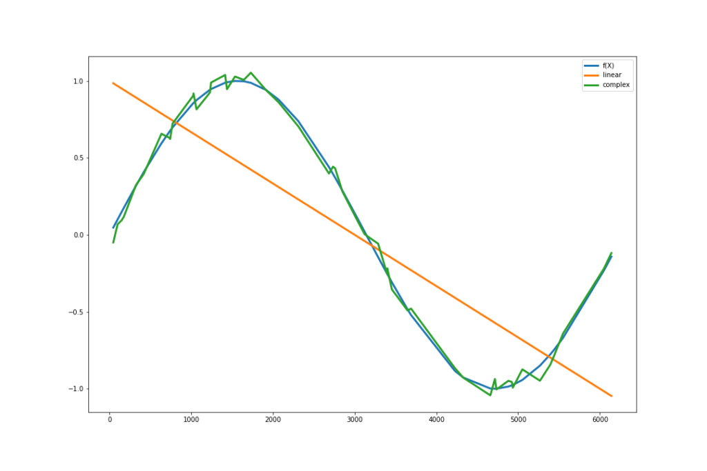
In the above image, I tried to model the sin curve ( $f(X)$ ) with two models models. First one (linear)d with two parameters ( $slope$ and $intercept$ ) while the second one (complex) is sin curve plus some Gaussian noise. if we take a sample – let’s say 100 – data points from sin curve and plug in these values in the bias-variance expressions above, we get the following:

	Linear	Complex
Bias	0.50	0.50
Variance	0.37	0.51

You can take any toy example like this and try it out yourself. Check how bias and variance changes if we change model complexity.

Part II: Not so formal derivation

Now let’s look at the derivation for bias variance decomposition for the regression problems. We can use similar approach in classification as well, as we have already discussed.

$\begin{aligned} \overbrace{E[(y- \hat{f}(X))^2]}^{MSE} &= E[y^2 - 2y\hat{f}(X) + \hat{f}(X)^2] \\ &= E[y^2] + E[\hat{f}(X)^2] - 2E[y\hat{f}(X)] \end{aligned}$

We defined $y = f(X) + \epsilon$

$\begin{aligned} E[y^2] &= E[(f(X) + \epsilon)^2] \\ &= E[f(X)^2] + 2E[f(X).\epsilon] + \underbrace{E[\epsilon^2]}_{Noise} \\ &= f(X)^2 + 2f(X).E[\epsilon] + \sigma^2 & \because f(X)\ doesn't\ depend\ on\ the\ data \\ &= f(X)^2 + \sigma^2 & \because E[\epsilon]=0\ and\ E[\epsilon^2]=\sigma^2 \end{aligned}$

Now looking at the second term $E[\hat{f}(X)^2]$

$\begin{aligned} E[\hat{f}(X)^2] = \overbrace{E[(\hat{f}(X) - E[\hat{f}(X)])^2]}^{Variance} + E[\hat{f}(X)]^2 \\ \because Var[X] = E[(X - E[X])^2] = E[X^2] - E[X]^2 \end{aligned}$

Lastly looking at the covariance term

$\begin{aligned} E[y.\hat{f}(X)] &= E[(f(X) + \epsilon).\hat{f}(X)] & \because y = f(X) + \epsilon \\ &= E[f(X).\hat{f}(X)] + E[\epsilon.\hat{f}(X)] \\ &= f(X).E[\hat{f}(X)] + E[\epsilon].E[\hat{f}(X)] & \because \hat{f}(X)\ and\ \epsilon\ are\ independent \\ &= f(X).E[\hat{f}(X)] & \because E[\epsilon] = 0 \end{aligned}$

Plugging all of them together

$\begin{aligned} MSE &= f(X)^2 + \sigma^2 + E[(\hat{f}(X) - E[\hat{f}(X)])^2] + E[\hat{f}(X)]^2 - 2f(X).E[\hat{f}(X)] \\ &= \underbrace{(E[\hat{f}(X)] - f(X))^2}_{Bias^2} + \sigma^2 + E[(\hat{f}(X) - E[\hat{f}(X)])^2] \\ \end{aligned}$

Thus we can say $MSE = Bias^2 + Variance + Noise$ , Also note that:

$\begin{aligned} \overbrace{E[(y- \hat{f}(X))^2]}^{MSE} &= E[(f(X) + \epsilon - \hat{f}(X))^2] \\ &= \underbrace{E[(f(X) - \hat{f}(X))^2]}_{True Error} - 2E[\epsilon.(f(X) - \hat{f}(X))] + E[\epsilon^2]\\ \end{aligned}$

Here again the middle term will go to 0 since $\epsilon$ is independent of the true error
And we can further show that $True Error = Bias^2 + Variance$ .

Final thoughts

We need to consider the bias and variance of our model in order to choose one which generalizes well and fits appropriately to the data. Bias and variance will be different based on the data distributions, machine learning problem (regression, classification etc.), Algorithm used for modelling the data. Here we just looked at the mathematical intuition behind the Bias and variance, which will help us in engineering our models better. you should also check out Wikipedia page of Bias-Variance.

There are more things we can look into to really make our understanding of Bias and variance better, like:

How to treat high bias?
How to treat high Variance?
What is regularization?
How is regularization is related to bias and variance (mathematically and intuitively both)?
What are different regularization strategies with respect to data distribution, ML algorithms and ML paradigm?
What regularization strategy to use and when?

Let me know if you want me to write a blog on any of these topics. Also feel free to discuss it in comments.

Base Zero