Introduction
In a world increasingly obsessed with complex neural networks and black-box algorithms, there’s something almost rebellious about the elegant simplicity of linear regression. Like the opening riff of “Smoke on the Water” or the geometric precision of a Kubrick frame, linear regression represents that rare intersection of mathematical beauty and practical utility. It’s the statistical equivalent of Occam’s razor—why make things complicated when a straight line might just do the trick?
Linear regression remains the workhorse of statistical modeling, the foundation upon which entire careers in data science are built. From predicting housing prices to understanding the relationship between advertising spend and sales, this deceptively simple technique continues to deliver insights that would make even the most sophisticated deep learning models blush with envy.
Background & Historical Foundations
The story of linear regression begins not in Silicon Valley, but in 19th century Europe with two mathematical titans: Carl Friedrich Gauss and Adrien-Marie Legendre. Both independently developed the method of least squares around 1805-1809, though Gauss claimed priority based on earlier unpublished work (Stigler, 1981). Their breakthrough was recognizing that the “best” line through a set of points minimizes the sum of squared vertical distances—a concept so fundamental it feels almost obvious in retrospect.
The term “regression” itself comes from Francis Galton’s 1886 study of heredity, where he observed that extreme characteristics (like height) tend to “regress” toward the mean in subsequent generations. This phenomenon, now known as regression toward the mean, gave the technique its name despite the method being fundamentally about prediction rather than literal regression.
Core Concepts: The Mathematical Machinery
The Simple Linear Model
At its heart, simple linear regression models the relationship between two variables:
y = β₀ + β₁x + ε
Where:
- y is the dependent variable (what we’re trying to predict)
- x is the independent variable (our predictor)
- β₀ is the y-intercept
- β₁ is the slope coefficient
- ε is the error term (what we can’t explain)
Ordinary Least Squares (OLS) Estimation
The OLS method finds the coefficients that minimize the sum of squared residuals:
min Σ(yᵢ – ŷᵢ)²
Where ŷᵢ = β₀ + β₁xᵢ is our predicted value. The solution gives us:
β₁ = Σ(xᵢ – x̄)(yᵢ – ȳ) / Σ(xᵢ – x̄)²
β₀ = ȳ – β₁x̄
Multiple Linear Regression
When life gives you more than one predictor variable, multiple linear regression comes to the rescue:
y = β₀ + β₁x₁ + β₂x₂ + … + βₚxₚ + ε
The OLS solution becomes more complex, involving matrix algebra:
β = (XᵀX)⁻¹Xᵀy
Where X is the design matrix containing our predictor variables.
The Four Pillars: Assumptions of Linear Regression
Like any good statistical method, linear regression comes with assumptions—break them at your peril:
1. Linearity
The relationship between predictors and response should be linear. Violations here are like trying to fit a square peg in a round hole—it might go in, but it won’t be pretty.
2. Independence
Observations should be independent of each other. Time series data, for example, often violates this assumption due to autocorrelation.
3. Homoscedasticity
The variance of errors should be constant across all levels of the predictors. Heteroscedasticity (the opposite) makes your standard errors unreliable.
4. Normality
Errors should be normally distributed. This matters most for small sample sizes and hypothesis testing.
Practical Applications & Implementation
Real-World Use Cases
Linear regression shines in numerous domains:
- Economics: Predicting GDP growth based on various indicators
- Healthcare: Estimating patient recovery time based on treatment variables
- Marketing: Understanding how advertising spend affects sales
- Real Estate: Predicting house prices from square footage, location, etc.
Python Implementation Example
import numpy as np
import pandas as pd
import statsmodels.api as sm
from sklearn.linear_model import LinearRegression
from sklearn.model_selection import train_test_split
from sklearn.metrics import r2_score, mean_squared_error

# Generate sample data
np.random.seed(42)
X = np.random.randn(100, 3)  # 3 features
y = 2.5 + 1.5*X[:,0] + 0.8*X[:,1] - 1.2*X[:,2] + np.random.randn(100)*0.5

# Using statsmodels for detailed output
X_with_const = sm.add_constant(X)
model = sm.OLS(y, X_with_const)
results = model.fit()
print(results.summary())

# Using scikit-learn for prediction
X_train, X_test, y_train, y_test = train_test_split(X, y, test_size=0.2)
lr = LinearRegression()
lr.fit(X_train, y_train)
predictions = lr.predict(X_test)

print(f"R-squared: {r2_score(y_test, predictions):.3f}")
print(f"MSE: {mean_squared_error(y_test, predictions):.3f}")
Challenges & Pitfalls
Multicollinearity: The Silent Assassin
When predictor variables are highly correlated, multicollinearity rears its ugly head. It doesn’t bias your predictions, but it makes coefficient estimates unstable and hard to interpret. The Variance Inflation Factor (VIF) helps detect it:
VIF = 1 / (1 – R²ⱼ)
Where R²ⱼ is the R-squared from regressing the j-th predictor on all other predictors. VIF > 5-10 suggests problematic multicollinearity.
Overfitting: The Siren’s Song
Adding too many variables can lead to overfitting—your model looks great on training data but fails miserably on new data. Regularization techniques like Ridge or Lasso regression help combat this.
The Curse of Interpretation
A common mistake is interpreting correlation as causation. Just because ice cream sales and drowning incidents are correlated doesn’t mean buying more ice cream causes more drownings (hello, summer heat).
Model Validation & Diagnostic Techniques
Residual Analysis
Plotting residuals against predicted values can reveal:
- Non-linearity (pattern in residuals)
- Heteroscedasticity (fan-shaped pattern)
- Outliers (points far from zero)
Cross-Validation
K-fold cross-validation helps assess how well your model generalizes to unseen data—the statistical equivalent of “trust, but verify.”
R-squared and Adjusted R-squared
While R² measures goodness-of-fit, it has a fatal flaw: it always increases with more variables. Adjusted R² penalizes additional variables, providing a more honest assessment.
Advantages Over Fancier Models
In an era where everyone wants to build neural networks, linear regression offers several advantages:
- Interpretability: You can actually understand what the coefficients mean
- Computational Efficiency: Trains in milliseconds, not hours
- Statistical Foundation: Well-understood properties and inference
- Baseline Performance: Often performs surprisingly well compared to more complex models
As the saying goes, “If you can’t explain it with linear regression, you probably don’t understand it well enough.”
Future Outlook & Extensions
Linear regression continues to evolve. Bayesian approaches incorporate prior knowledge, while generalized linear models (GLMs) extend the framework to non-normal error distributions. Quantile regression focuses on different parts of the response distribution rather than just the mean.
The future likely holds more hybrid approaches—combining linear models’ interpretability with neural networks’ flexibility. Because sometimes, you need both the straightforward honesty of a linear relationship and the complex nuance of deeper patterns.
Conclusion
Linear regression is the statistical equivalent of the three-chord rock song—seemingly simple, yet capable of profound expression in the right hands. It teaches us that sometimes the most powerful insights come not from complexity, but from understanding fundamental relationships clearly.
In a world increasingly dominated by algorithms we can’t understand, linear regression remains a beacon of transparency and interpretability. It reminds us that before we reach for the deep learning hammer, we should check if our problem is actually a nail that a simple straight line can solve.
As Gauss might say if he were alive today: sometimes the simplest solution is not just elegant—it’s true.
References
Stigler, S. M. (1981). Gauss and the Invention of Least Squares. The Annals of Statistics, 9(3), 465–474.
James, G., Witten, D., Hastie, T., & Tibshirani, R. (2013). An Introduction to Statistical Learning. Springer.
Montgomery, D. C., Peck, E. A., & Vining, G. G. (2012). Introduction to Linear Regression Analysis. John Wiley & Sons.
Fox, J. (2015). Applied Regression Analysis and Generalized Linear Models. Sage Publications.
Related posts:
 The Ultimate Guide to Machine Learning Algorithms: From Linear Regression to Neural Networks
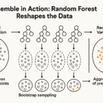 The Random Forest Revolution: Why Your Single Decision Tree Is Doomed to Fail
 The Unstoppable Force: How GBDT Ensemble Methods Conquer Machine Learning’s Toughest Battles
 The Unlikely Hero: How Naive Bayes Defies Expectations in Machine Learning
Leave a Reply