Introduction: Welcome to the Machine Learning Revolution

Machine learning isn’t just another buzzword thrown around by tech bros in Silicon Valley coffee shops – it’s the mathematical backbone of our modern digital existence. At its core, machine learning is the art and science of teaching computers to learn patterns from data without being explicitly programmed for every single scenario. It’s like teaching a child to recognize cats versus dogs rather than showing them every possible cat and dog picture in existence.

The Three Pillars of Machine Learning

Supervised Learning: Think of this as learning with training wheels. You provide the algorithm with labeled data (input-output pairs), and it learns to map inputs to outputs. It’s like showing a student exam questions with answers and then testing them on similar questions.

Unsupervised Learning: This is the wild west of machine learning. No labels, no guidance – just raw data waiting to reveal its hidden patterns. It’s like giving an archaeologist a pile of artifacts and asking them to categorize everything without any historical context.

Reinforcement Learning: The video game approach. An agent learns by interacting with an environment and receiving rewards or penalties. It’s how you taught yourself to not touch a hot stove after that one unfortunate childhood incident.

Understanding these algorithms isn’t just academic exercise – it’s the difference between throwing random algorithms at problems versus strategically selecting the right tool for the job. It’s the difference between a carpenter who knows only hammers and one with a complete toolbox.

Core Machine Learning Algorithms: Your Digital Toolkit

Linear Regression: The Foundation Stone

Intuition: Linear regression is the Oasis of machine learning – simple, straightforward, and surprisingly powerful. It finds the best-fitting straight line through your data points. If you’ve ever drawn a line through scattered points on graph paper, you’ve done linear regression manually.

Mathematical Formula:
y = mx + b (for simple linear regression)
Where:

• y = dependent variable
• x = independent variable
• m = slope
• b = y-intercept

For multiple variables: y = β₀ + β₁x₁ + β₂x₂ + ... + βₙxₙ

Example: Predicting house prices based on square footage. The algorithm learns that as square footage increases, price tends to increase in a linear fashion.

Logistic Regression: The Binary Classifier

Classification vs Regression: While linear regression predicts continuous values (like price), logistic regression predicts probabilities for binary outcomes (spam/not spam, cancer/not cancer).

Sigmoid Function: This S-shaped curve squashes any input into the 0-1 range, perfect for probability estimates. It’s the mathematical equivalent of a bouncer deciding who gets into the club (1) and who doesn’t (0).

Example: Email spam detection. The algorithm calculates the probability that an email is spam based on features like suspicious words, sender reputation, and formatting.

Decision Trees: The Flowchart Masters

Splitting Criteria: Decision trees use metrics like Gini impurity or information gain to determine the best features to split on. It’s like playing 20 questions – each question (split) should eliminate as many possibilities as possible.

Overfitting Issues: Decision trees can become so specific they memorize the training data rather than learning general patterns. It’s the difference between learning the concept of “dog” versus memorizing every dog you’ve ever seen.

Example: Loan approval decisions. The tree might first split on income, then credit score, then employment history, creating a clear path to approval or rejection.

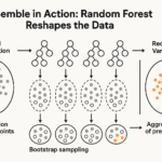
Random Forests: The Wisdom of Crowds

Ensemble Concept: Random forests combine multiple decision trees to create a more robust model. It’s like asking 100 experts for their opinion instead of trusting one potentially biased individual.

Bagging: Bootstrap aggregating creates multiple training datasets by sampling with replacement, then averages the predictions. It’s the machine learning equivalent of “measure twice, cut once.”

Feature Importance: Random forests can tell you which features are most important for predictions, adding interpretability to complex models.

Support Vector Machines: The Margin Maximizers

Margin Maximization: SVMs find the hyperplane that maximizes the margin between classes. They’re the bodyguards of machine learning – creating the biggest possible buffer zone between different groups.

Kernels: When data isn’t linearly separable, kernels transform it into higher dimensions where separation becomes possible. It’s like solving a 3D problem by thinking in 4D.

Example: Image classification where you need to separate different objects with clear boundaries.

K-Nearest Neighbors: The Lazy Learner

Distance Metric: KNN uses distance measures (Euclidean, Manhattan, etc.) to find the most similar data points. It assumes that similar things exist close to each other.

Lazy Learning: KNN doesn’t learn a model during training – it simply stores the data and computes distances during prediction. It’s the student who crams the night before the exam rather than studying throughout the semester.

Example: Recommender systems where “users who liked this also liked that” based on similarity.

Naïve Bayes: The Probability Purists

Bayes Theorem: This algorithm uses conditional probability to make predictions. It’s mathematically elegant but makes a strong assumption about feature independence.

Assumption of Independence: Naïve Bayes assumes all features contribute independently to the probability, which is rarely true but often works surprisingly well anyway.

Example: Text classification where words are treated as independent features contributing to document classification.

K-Means Clustering: The Grouping Guru

Centroid Initialization: K-means starts by randomly placing cluster centers, then iteratively improves them. The initial placement can significantly affect results – it’s like choosing starting positions in a game of musical chairs.

Convergence: The algorithm stops when cluster assignments stop changing or after a maximum number of iterations.

Example: Customer segmentation for marketing campaigns based on purchasing behavior and demographics.

Principal Component Analysis: The Dimension Reducer

Dimensionality Reduction: PCA finds the directions of maximum variance in high-dimensional data and projects it onto a lower-dimensional space. It’s like summarizing a 500-page book into its 10 most important themes.

Variance Capture: The goal is to retain as much information (variance) as possible while reducing dimensions.

Example: Visualizing high-dimensional data in 2D or 3D plots while preserving the most important patterns.

Neural Networks: The Brain Mimics

Perceptron: The basic building block of neural networks, inspired by biological neurons. It takes weighted inputs, sums them, and applies an activation function.

Layers: Neural networks consist of input layers, hidden layers, and output layers. Each layer transforms the data in increasingly complex ways.

Activation Functions: Functions like ReLU, sigmoid, and tanh introduce non-linearity, allowing networks to learn complex patterns.

Example: Handwriting recognition where the network learns to recognize patterns in pixel data.

Reinforcement Learning: The Trial and Error Expert

Agent-Environment Interaction: The agent takes actions in an environment and receives rewards or penalties. It’s the digital equivalent of training a dog with treats.

Reward System: The agent learns to maximize cumulative reward over time, often using techniques like Q-learning or policy gradients.

Example: Game playing AI that learns optimal strategies through millions of gameplay iterations.

Practical Examples: Code That Actually Works

Let’s get our hands dirty with some Python code using scikit-learn. I’ll show you examples that actually run rather than theoretical pseudocode.

Linear Regression Example: Predicting House Prices

import numpy as np
from sklearn.linear_model import LinearRegression
from sklearn.model_selection import train_test_split
from sklearn.metrics import mean_squared_error
import matplotlib.pyplot as plt

# Sample data: square footage vs price
X = np.array([[600], [800], [1000], [1200], [1400], [1600]])  # Square footage
y = np.array([150000, 200000, 250000, 300000, 350000, 400000])  # Price

# Split data
X_train, X_test, y_train, y_test = train_test_split(X, y, test_size=0.2, random_state=42)

# Create and train model
model = LinearRegression()
model.fit(X_train, y_train)

# Predict and evaluate
predictions = model.predict(X_test)
mse = mean_squared_error(y_test, predictions)
print(f"Mean Squared Error: {mse:.2f}")
print(f"Coefficient: {model.coef_[0]:.2f}")
print(f"Intercept: {model.intercept_:.2f}")

# Plot results
plt.scatter(X, y, color='blue')
plt.plot(X, model.predict(X), color='red')
plt.xlabel('Square Footage')
plt.ylabel('Price')
plt.title('House Price Prediction')
plt.show()

Logistic Regression Example: Iris Classification

from sklearn.datasets import load_iris
from sklearn.linear_model import LogisticRegression
from sklearn.model_selection import train_test_split
from sklearn.metrics import accuracy_score, confusion_matrix
import seaborn as sns

# Load famous Iris dataset
iris = load_iris()
X, y = iris.data, iris.target

# Split data
X_train, X_test, y_train, y_test = train_test_split(X, y, test_size=0.3, random_state=42)

# Create and train model
model = LogisticRegression(max_iter=200)
model.fit(X_train, y_train)

# Predict and evaluate
predictions = model.predict(X_test)
accuracy = accuracy_score(y_test, predictions)
print(f"Accuracy: {accuracy:.2f}")

# Confusion matrix
cm = confusion_matrix(y_test, predictions)
sns.heatmap(cm, annot=True, fmt='d')
plt.xlabel('Predicted')
plt.ylabel('Actual')
plt.title('Confusion Matrix')
plt.show()

Algorithm Comparison: Choosing Your Weapon

Strengths and Weaknesses Summary

Linear Regression

• Strengths: Simple, fast, interpretable, works well with linear relationships
• Weaknesses: Poor with non-linear data, sensitive to outliers

Logistic Regression

• Strengths: Probabilistic outputs, fast training, good for binary classification
• Weaknesses: Linear decision boundary, requires feature scaling

Decision Trees

• Strengths: Easy to interpret, handles non-linear data, feature importance
• Weaknesses: Prone to overfitting, unstable (small data changes affect structure)

Random Forests

• Strengths: Reduces overfitting, handles high dimensions, feature importance
• Weaknesses: Computationally expensive, less interpretable than single trees

Support Vector Machines

• Strengths: Effective in high dimensions, versatile with kernels, good with clear margins
• Weaknesses: Computationally intensive, sensitive to parameters, poor with noisy data

K-Nearest Neighbors

• Strengths: Simple implementation, no training time, adapts to new data
• Weaknesses: Computationally expensive prediction, sensitive to irrelevant features

Decision Guideline: When to Use What

Use Regression When:

• Predicting continuous values (prices, temperatures, quantities)
• Relationships are approximately linear
• Interpretability is important

Use Trees When:

• You need interpretable decisions
• Data has non-linear relationships
• Feature importance analysis is needed

Use SVM When:

• You have clear margins between classes
• Dealing with high-dimensional data
• Need strong theoretical guarantees

Use Clustering When:

• Exploring unknown patterns in data
• Segmenting customers or products
• Dimensionality reduction needed

Use Neural Networks When:

• Dealing with complex patterns (images, speech, text)
• Have large amounts of data
• Other algorithms aren’t performing well

Conclusion: Your Machine Learning Journey Begins Here

Understanding machine learning algorithms is like learning the grammar of a new language – it’s the foundation upon which you’ll build everything else. These algorithms aren’t just mathematical curiosities; they’re the tools that power everything from your Netflix recommendations to medical diagnosis systems.

Recommended Resources

Books:

• “Introduction to Statistical Learning” by Gareth James et al. (the friendly version)
• “Pattern Recognition and Machine Learning” by Christopher Bishop (the serious version)
• “Hands-On Machine Learning with Scikit-Learn and TensorFlow” by Aurélien Géron (the practical version)

Courses:

• Andrew Ng’s Machine Learning course on Coursera (the classic)
• Fast.ai practical deep learning courses (the modern approach)
• Stanford CS229 lectures (the mathematical deep dive)

Datasets to Practice With:

• UCI Machine Learning Repository (the granddaddy of them all)
• Kaggle datasets (with community and competitions)
• Scikit-learn built-in datasets (perfect for beginners)

The most important step isn’t reading about these algorithms – it’s implementing them. Fire up Jupyter Notebook, load some data, and start experimenting. Make mistakes, break things, and learn from the process. The difference between someone who understands machine learning and someone who just talks about it is the willingness to get their hands dirty with code.

Remember what Kubrick said about filmmaking – it’s not about having the right answers, but about asking the right questions. In machine learning, the algorithms are your tools, but the real art is in framing the problems and interpreting the results.

Now go build something interesting.