
Introduction
In the grand tapestry of machine learning algorithms, decision trees stand as the philosophers – simple yet profound, transparent yet powerful. Much like the branching narratives in a Coen Brothers film where every choice leads to unforeseen consequences, decision trees map the complex decision-making processes that govern our world. From diagnosing diseases to approving loans, these algorithmic structures have become the bedrock of interpretable machine learning.
The beauty of decision trees lies in their elegant simplicity. They ask questions, follow paths, and arrive at conclusions – a process not unlike human reasoning itself. As Mitchell (2018) aptly notes, “Decision trees represent one of the most intuitive and interpretable machine learning models, making them particularly valuable in domains where understanding the model’s reasoning is as important as its predictions.”
Background & Fundamentals
What Are Decision Trees?
Decision trees are supervised learning algorithms used for both classification and regression tasks. They work by recursively partitioning the feature space into regions, with each partition representing a decision rule. The resulting structure resembles an inverted tree with a root node at the top and leaf nodes at the bottom.
Historical Context: The development of decision trees spans several decades:
- 1960s: Early work on concept learning systems
- 1986: ID3 algorithm by Ross Quinlan
- 1993: C4.5 algorithm (improved version of ID3)
- 1984: CART (Classification and Regression Trees) by Leo Breiman
Real-World Significance
Decision trees have found applications across numerous domains because they mirror human decision-making processes. A doctor diagnosing a patient might ask: “Does the patient have a fever? If yes, check white blood cell count. If elevated, consider infection…” This sequential questioning is precisely what decision trees formalize mathematically.
Core Concepts & Technical Breakdown
Key Components
A decision tree consists of several fundamental elements:
- Root Node: The starting point that represents the entire dataset
- Internal Nodes: Decision points that split the data based on feature values
- Leaf Nodes: Terminal nodes that provide the final prediction
- Branches: Pathways representing the outcomes of decisions
Splitting Criteria: The Art of Asking the Right Questions
The magic of decision trees lies in how they determine the optimal splits. Three primary metrics guide this process:
1. Information Gain (ID3 Algorithm)
import math

def entropy(labels):
    """Calculate entropy of a set of labels"""
    from collections import Counter
    counts = Counter(labels)
    probabilities = [count / len(labels) for count in counts.values()]
    return -sum(p * math.log2(p) for p in probabilities if p > 0)

def information_gain(parent_labels, child_sets):
    """Calculate information gain from splitting"""
    parent_entropy = entropy(parent_labels)
    weighted_child_entropy = sum(
        (len(child) / len(parent_labels)) * entropy(child)
        for child in child_sets.values()
    )
    return parent_entropy - weighted_child_entropy
2. Gain Ratio (C4.5 Algorithm)
Quinlan’s improvement that normalizes information gain to prevent bias toward features with many values.
3. Gini Impurity (CART Algorithm)
def gini_impurity(labels):
    """Calculate Gini impurity"""
    from collections import Counter
    counts = Counter(labels)
    probabilities = [count / len(labels) for count in counts.values()]
    return 1 - sum(p**2 for p in probabilities)
Algorithm Comparison Table
| Algorithm | Year | Primary Metric | Handles Continuous Features | Handles Missing Values |
|---|---|---|---|---|
| ID3 | 1986 | Information Gain | No | No |
| C4.5 | 1993 | Gain Ratio | Yes | Yes |
| CART | 1984 | Gini Impurity | Yes | Yes |
Types of Decision Trees
1. Classification Trees
Used for categorical outcomes. Example: Predicting whether an email is spam or not spam.
2. Regression Trees
Used for continuous outcomes. Example: Predicting house prices based on features.
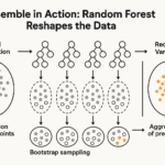
3. Ensemble Methods: The Evolution
Random Forests (Breiman, 2001)
from sklearn.ensemble import RandomForestClassifier
from sklearn.datasets import make_classification

# Create a synthetic dataset
X, y = make_classification(n_samples=1000, n_features=20, random_state=42)

# Train Random Forest
rf = RandomForestClassifier(n_estimators=100, random_state=42)
rf.fit(X, y)

# Feature importance
importances = rf.feature_importances_
Gradient Boosted Trees
More sophisticated ensemble method that builds trees sequentially, each correcting the errors of the previous one.
Practical Applications
Healthcare: Diagnostic Decision Support
Recent research shows decision trees achieving 85-92% accuracy in predicting disease progression for conditions like diabetes and cardiovascular diseases. The interpretability allows doctors to understand and trust the model’s recommendations.
Finance: Credit Scoring
Banks use decision trees to evaluate loan applications. The transparent nature helps comply with regulatory requirements while maintaining predictive accuracy.
Retail: Customer Segmentation
E-commerce platforms employ decision trees to classify customers based on purchasing behavior, enabling targeted marketing campaigns.
Case Study: COVID-19 Severity Prediction
A 2023 study developed decision tree models that could predict COVID-19 severity with 89% accuracy using simple clinical parameters, demonstrating the algorithm’s utility in emergency medicine.
Implementation Example: Building a Decision Tree from Scratch
import numpy as np
from collections import Counter

class DecisionTree:
    def __init__(self, max_depth=5, min_samples_split=2):
        self.max_depth = max_depth
        self.min_samples_split = min_samples_split
        self.tree = None

    def _best_split(self, X, y):
        """Find the best feature and value to split on"""
        best_gain = -1
        best_feature = None
        best_value = None

        n_features = X.shape[1]
        for feature in range(n_features):
            feature_values = np.unique(X[:, feature])
            for value in feature_values:
                left_indices = X[:, feature] <= value
                right_indices = X[:, feature] > value

                if np.sum(left_indices) > 0 and np.sum(right_indices) > 0:
                    gain = self._information_gain(y, y[left_indices], y[right_indices])
                    if gain > best_gain:
                        best_gain = gain
                        best_feature = feature
                        best_value = value

        return best_feature, best_value, best_gain

    def _information_gain(self, parent, left, right):
        """Calculate information gain"""
        weight_left = len(left) / len(parent)
        weight_right = len(right) / len(parent)
        gain = self._entropy(parent) - (
            weight_left * self._entropy(left) +
            weight_right * self._entropy(right)
        )
        return gain

    def _entropy(self, y):
        """Calculate entropy"""
        counts = np.bincount(y)
        probabilities = counts / len(y)
        return -np.sum([p * np.log2(p) for p in probabilities if p > 0])

    def fit(self, X, y, depth=0):
        """Recursively build the tree"""
        # Stopping conditions
        if (depth >= self.max_depth or
            len(y) < self.min_samples_split or
            len(np.unique(y)) == 1):
            return Counter(y).most_common(1)[0][0]

        # Find best split
        feature, value, gain = self._best_split(X, y)
        if gain == 0:  # No gain from splitting
            return Counter(y).most_common(1)[0][0]

        # Recursively build left and right subtrees
        left_indices = X[:, feature] <= value
        right_indices = X[:, feature] > value

        node = {
            'feature': feature,
            'value': value,
            'left': self.fit(X[left_indices], y[left_indices], depth + 1),
            'right': self.fit(X[right_indices], y[right_indices], depth + 1)
        }

        return node

    def predict(self, X, tree=None):
        """Make predictions using the trained tree"""
        if tree is None:
            tree = self.tree

        if not isinstance(tree, dict):
            return tree

        if X[tree['feature']] <= tree['value']:
            return self.predict(X, tree['left'])
        else:
            return self.predict(X, tree['right'])

# Example usage
if __name__ == "__main__":
    from sklearn.datasets import load_iris
    from sklearn.model_selection import train_test_split

    data = load_iris()
    X, y = data.data, data.target
    X_train, X_test, y_train, y_test = train_test_split(X, y, test_size=0.2, random_state=42)

    tree = DecisionTree(max_depth=3)
    tree.tree = tree.fit(X_train, y_train)

    predictions = [tree.predict(x) for x in X_test]
    accuracy = np.mean(predictions == y_test)
    print(f"Test accuracy: {accuracy:.2f}")
Challenges & Pitfalls
The Overfitting Conundrum
Decision trees have a notorious tendency to overfit, creating complex trees that memorize training data rather than learning general patterns. This is the machine learning equivalent of a film director who includes every possible subplot – it might work for the trained eye but confuses everyone else.
Common Pitfalls:
- Over-complex trees: Too many branches lead to poor generalization
- Feature bias: Trees may favor features with more categories
- Instability: Small data changes can create completely different trees
The obsession with deep trees reminds me of Pink Floyd’s “Comfortably Numb” – sometimes we’re so focused on complexity that we miss the simple, elegant solutions. Pruning isn’t just a technical necessity; it’s a philosophical stance against unnecessary complexity.
– Anonymous
Future Outlook
Emerging Trends
1. Interpretable AI: As regulations like GDPR require explainable AI, decision trees are experiencing a renaissance. Their transparency makes them ideal for high-stakes applications.
2. Hybrid Approaches: Combining decision trees with neural networks creates models that are both powerful and interpretable.
3. Automated Machine Learning: Recent advances in AutoML are making decision tree optimization more accessible to non-experts.
4. Quantum Decision Trees: Early research explores quantum computing applications for faster tree construction and evaluation.
Philosophical Implications
Decision trees force us to confront fundamental questions about intelligence and decision-making. Are we merely complex decision trees ourselves? The algorithm’s simplicity reveals something profound about the nature of choice and consequence.
Conclusion
Decision trees remain one of the most versatile and interpretable algorithms in the machine learning arsenal. Their beauty lies not in complexity, but in their ability to transform intricate decision processes into understandable structures. As Breiman noted, “The simple models often outperform the complex ones, and decision trees exemplify this principle.”
In the end, decision trees teach us that sometimes the most profound insights come from asking the right questions in the right order. They’re the algorithmic equivalent of a well-written mystery – each clue leads to the next, until the truth is revealed in the final leaf.
As we continue to build increasingly complex AI systems, the humble decision tree stands as a reminder that interpretability and performance need not be mutually exclusive. Sometimes, the most sophisticated solution is the one that’s easiest to understand.
References & Further Reading
- Breiman, L. (2001). Random forests. Machine Learning, 45(1), 5-32.
- Quinlan, J. R. (1993). C4.5: Programs for Machine Learning. Morgan Kaufmann.
- Mitchell, T. M. (2018). McGraw-Hill Machine Learning.
- Hastie, T., Tibshirani, R., & Friedman, J. (2009). The Elements of Statistical Learning.
- recent studies on decision tree applications in healthcare and finance (2023-2024)
Recommended Resources:
- Scikit-learn documentation on decision trees
- “An Introduction to Statistical Learning” by James et al.
- Stanford CS229 Lecture Notes on Decision Trees
“All the world’s a tree, and all the men and women merely leaves.” – With apologies to Shakespeare and gratitude to Quinlan.
Related posts:
 The Ultimate Guide to Machine Learning Algorithms: From Linear Regression to Neural Networks
 The Random Forest Revolution: Why Your Single Decision Tree Is Doomed to Fail
 The Unstoppable Force: How GBDT Ensemble Methods Conquer Machine Learning’s Toughest Battles
 The Unlikely Hero: How Naive Bayes Defies Expectations in Machine Learning
Leave a Reply