
In the world of AI its more or less straight forward to deal with data which is inherently represented by numbers, but in case of text things start to get tricky. Word2Vec published in Distributed representations of words phrases and their compositionality (Mikolov et al) was a major breakthrough as they were able to create vector representation of words which captured their meaning and can be further used for other Machine learning or AI downstream tasks.
Although they weren’t the first to do it but they made it efficient to compute. In this blog I’ll cover Skip-gram with negative sampling (one of the efficient ways to compute word vectors suggested in Mikolov et al) and how to create your own Word2Vec model using pytorch.
What are word vectors?
As we know that machine learning algorithms or the computer per se understands number not words. To make our algorithm understand words we need to represent them as numbers or vectors. Also they should make sense – i.e. they must capture information about words like their meaning, part of speech, connotation etc. – so that our algorithm can learn to perform this encoded information.
These vector representation of words can be of two types:
- Sparse (One hot vector): Its a huge vector of length of the vocabulary of words with all zeros except index of the word in the vocabulary – which is one. Its extremely inefficient way of representing a word, plus the size of vector is huge and you have to maintain two hash map – mapping word and their indices and vice versa.
- Dense (Word2Vec): These are word representation which solves all the caveats of the sparse vectors. They can be learned by Singular value decomposition (SVD) of Pointwise mutual information (PMI) of words or using deep learning.
In this blog I’ll walk you through one of the deep learning based approach to learn these vectors called Word2Vec.
How to create word representations
you shall know a word by the company it keeps.
John Rupert Firth
There are several ways to do it using both good old machine learning and state-of-the-art deep learning. As we already discussed running a dimensionality reduction algorithm over PMI matrix of words is more traditional way to do it. PMI is a VxV matrix where V is the size of the vocabulary. Each element of this matrix is filled with probability of co-occurrence of the pair of words. Since this will again be a huge sparse matrix we reduce its dimensionality to get our word embedding.
Its not mandatory to just look at the pair of words for co-occurrence i.e. 2-gram we can extend this approach to n-gram which is n word window around the word of interest.
In deep learning we don’t have to explicitly compute PMI matrix. We just give one hot encoded input and predict one hot encoded output with one input layer in between. The network is trained using Cross-Entropy loss. There are two main approach that I want to mention:
- Continuous bag of words: We predict
nthword givenn-1previous words using Softmax output. Its a multi-class classification problem.
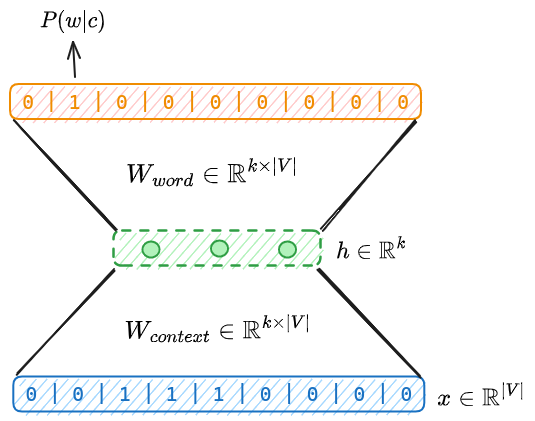
![\[L(\theta) = -\log(\hat{y}_{w)}= -\log P(w|c)\]](https://basezero.org.in/wp-content/ql-cache/quicklatex.com-2ff991b9b80a75a58d6e8a45bb8cebdf_l3.png "Rendered by QuickLaTeX.com")
![\[\hat{y}_{w} = \frac{exp(u_c. v_w)}{\sum_{w' \in W} exp(u_c . v_w)}\]](https://basezero.org.in/wp-content/ql-cache/quicklatex.com-8c732eb4b30d9e87b070d8a8c3513f2a_l3.png "Rendered by QuickLaTeX.com")
![\[u_{c} = W_{context} . x_c\]](https://basezero.org.in/wp-content/ql-cache/quicklatex.com-ba948d2fc353b5da717516f10bf62948_l3.png "Rendered by QuickLaTeX.com")
 is column of
- Skip-gram: Here we consider a window (context) of let say
cwords on both sides of the word of interest and predict the context words given the word. Just the opposite of CBoW.

![\[\underset{\theta}{\text{maximize}} \frac{1}{T} \sum_{t=1}^{T} \sum_{-c \le j \le c,j\ne0} \log p(w_{t+j} | w_t)\]](https://basezero.org.in/wp-content/ql-cache/quicklatex.com-f5daed838e4ec107991bc367d269b17b_l3.png "Rendered by QuickLaTeX.com")
![\[p(w_O | w_I) = \frac{exp({v'_{w_O}}^T v_{w_I})}{\sum_{w=1}^{W} exp(v'_w v_{w_I})}\]](https://basezero.org.in/wp-content/ql-cache/quicklatex.com-c1df4ff20f6a1c6654b9b63634822f00_l3.png "Rendered by QuickLaTeX.com")
Here  and
and  are representations of input and output words respectively, and
  is the number of words in the vocabulary.
Challenges associated with learning word representations
Both the formulations Continuous bag of words and Skip-gram, though they perform better than SVD approach, they rely on Softmax computation which is expensive. In Mikolov et al they addressed this problem and suggested three variations of Skip-gram model which are more efficient to compute:
- Hierarchical Softmax: Its computationally efficient approximation of full Softmax. It uses a binary tree representation of the output layer with
Wwords as leaf nodes. - Negative sampling: It uses a contrastive loss function which maximizes the probability of context words and reduces the probability of a sample of non context words (negative samples). It can be shown that this approach maximize the log probability of Softmax.
- Sub-sampling of frequent words: The frequent words like “the”, “an” etc. carry less information about the meaning of the words. The idea here is sub-sample such words while learning word representation.
In this blog we’ll look at the Skip-gram with negative sampling which is more commonly used technique to learn Word representations.
How Word2Vec helps?
As we’ve already seen that Skip-gram with negative sampling (Word2Vec) uses a contrastive loss function instead of Softmax. That’s the heart of this algorithm which makes it super efficient to train distributed representations of words. Let’s break down its loss function:
![\[\underset{\theta}{\text{maximize}} \sum_{(w,c) \in D} \log \sigma(v_c^Tv_w) + \sum_{(w,r) \in D'} \log \sigma(-v_r^Tv_w)\]](https://basezero.org.in/wp-content/ql-cache/quicklatex.com-1b68a5b6e6954f29eebec4370c9fc91f_l3.png "Rendered by QuickLaTeX.com")
![\[\sigma(x) = \frac{1}{1+e^{-x}}\]](https://basezero.org.in/wp-content/ql-cache/quicklatex.com-2459d8174ccc292f8b16e7ea2848738e_l3.png "Rendered by QuickLaTeX.com")
Here  , and
, and  are context, word and negative sample vector representations respectively. We’re not computing Softmax over the dot product of word vector with all other word vectors
  , but in this case we’re just computing the Sigmoid over dot product of word with context words and negative samples. This improved the training efficiency by 2X-10X.
Skip-gram with negative sampling using pytorch
I’ll break down the different parts of Word2Vec scripts for you to understand. In case you want the complete code you can checkout my github page. Clone it, fork it, give it a star if you like.
Project folder structure
Root folder is “Word2Vec” which contains:
- Artifacts: for saving processed data, models, plots and other artifacts.
- Data: containing raw data
- main.py: main file, but its better to use Word2Vec training and evaluation file in the notebooks folder
- src: contains utils.py and models.py files with all the source code.
- utils.py has two classes DataIO for data read and write, DataLoader for creating batches and negative samples.
- models.py has three classes SGNS – the model per se, Word2Vec – model training wrapper and EvaluateSGNS – to evaluate models.
Word2Vec
├── Artifacts
│   ├── metadata
│   └── model
├── Data
│   ├── ds1.txt
│   └── ds2.txt
├── ds2_coding.pdf
├── __init__.py
├── main.py
├── Mikolov et al.pdf
├── notebooks
│   └── Word2Vec training and evaluation.ipynb
├── __pycache__
│   └── main.cpython-311.pyc
├── setup.py
├── src
│   ├── models.py
│   ├── __pycache__
│   └── utils.py
Utils.py
class DataIO:
    def __init__(self, root_dir:str, filepath: List[str], vocab_size=10000):
        self.root_dir = root_dir
        self.vocab_size = vocab_size
        self.data = list()
        for file in filepath:
            path = os.path.join(root_dir, file)
            with open(path, 'r') as f:
                self.data.extend(f.read().strip().split())

    def get_metadata(self):
        word_counts = Counter(self.data).most_common(self.vocab_size-1)
        word2index = dict()

        for i, word in enumerate(word_counts):
            word2index[word[0]] = i

        unk_index = len(word2index)
        word2index['<UNK>'] = unk_index
        index2word = {v:k for k, v in word2index.items()}

        unk_count = 0
        processed_data = list()
        for word in self.data:
            if word in word2index:
                idx = word2index[word]
            else:
                idx = unk_index
                unk_count += 1
            processed_data.append(idx)
        word_counts.append(('<UNK>', unk_count))
        word_counts = [el[1] for el in word_counts]

        return processed_data, word_counts, word2index, index2word
DataIO class takes in list of text files, vocab size and root directory as input. It has a get_metadata function which returns word counts, word to index and index to word maps along with processed data which contains word indices instead of word per se.
I have set vocab size to 10000 which is quite low. You can play around with this parameter. This parameter is used to create word embedding for 10000 most frequent words rest of words are represented as ‘<UNK>’ token.
class DataLoader:
def __init__(self, data, word_counts, word2index, index2word, exp_const):
self.data = data
self.data_indices = np.arange(len(data))
self.word_counts = word_counts
self.indices = np.arange(len(word_counts))
self.N = sum(word_counts)
self.p_word = np.array(list(map(lambda count: math.pow(count, exp_const)/self.N, word_counts)))
self.p_word /= self.p_word.sum()
self.word2index = word2index
self.index2word = index2word
def get_negative_sample(self, inputs, k):
samples = list()
for word in inputs:
sample = list()
i = 0
while i &amp;amp;lt; k:
wr = np.random.choice(self.indices, p=self.p_word, replace=False)
if wr != word[0]:
i += 1
sample.append(wr)
samples.append(sample)
return np.array(samples)
def get_batch(self, window, batch_size):
outputs = np.zeros(shape=(batch_size, 2*window), dtype=int)
inputs = np.zeros(shape=(batch_size, 1), dtype=int)
i = 0
while i &amp;amp;lt; batch_size:
try:
wi = np.random.choice(self.data_indices, size=1)
idx = wi[0]
np.append(inputs, [self.data[idx]])
wo = self.data[idx+1:idx+window+1].extend(self.data[idx-window:idx])
np.append(outputs, wo)
i+=1
except:
continue
return inputs, outputs
def get_word(self, idx):
return self.index2word[idx]
def get_index(self, word):
return self.word2index[word]
DataLoader has two major functions get_batch and get_negative_sample:
- get_batch: It takes in window size and batch size as input and returns input (word) and output (context) indices.
- get_negative_sample: On the other hand this function takes input indices and number of negative samples as input and returns indices of negative samples.
The negative samples are drawn from a probability distribution  which is computed by normalizing the word counts raised to power lets say
  . Although in the original paper they found that
  works best.
models.py
class SGNS(nn.Module):
    def __init__(self, vocab_size, embedding_dim):
        super(SGNS, self).__init__()
        self.vocab_size = vocab_size
        self.embedding_dim = embedding_dim
        self.input_embedding = nn.Embedding(vocab_size, embedding_dim)
        self.output_embedding = nn.Embedding(vocab_size, embedding_dim)

    def forward(self, inputs, outputs, negative_sample):
        w_i = self.input_embedding(inputs)
        w_o = self.output_embedding(outputs)
        w_r = self.output_embedding(negative_sample)

        w_o = w_o.transpose(1,-1)
        w_r = w_r.transpose(1,-1)
        maximize_loss = torch.bmm(w_i, w_o).sigmoid().log().squeeze()
        minimize_loss = torch.bmm(w_i.negative(), w_r).sigmoid().log().sum(-1)

        return -(torch.add(maximize_loss, minimize_loss)).mean()

    def predict(self, inputs):
        return self.input_embedding(inputs)
SGNS class defines the architecture of the model. Forward function takes in input, output and negative samples as input and returns the loss, while predict function spits out the word vectors – it is supposed to be used after training the model.
class Word2Vec:
def __init__(
self,
root_dir,
train=True,
sgd=True,
process_data=False,
source_filepath=[],
metadata_filepath=None,
metadata_fnames=[],
vocab_size=10000,
embedding_dim=50,
exp_const=3/4,
learning_rate=1e-5
):
self.root_dir = root_dir
if process_data:
data_io = DataIO(root_dir, source_filepath, vocab_size)
data, word_counts, word2index, index2word = data_io.get_metadata()
else:
data, word_counts, word2index, index2word = DataIO.load_data(
root_dir,
metadata_filepath,
metadata_fnames
)
self.data_loader = DataLoader(
data,
word_counts,
word2index,
index2word,
exp_const
)
self.device = torch.device(&amp;amp;quot;cuda:0&amp;amp;quot; if torch.cuda.is_available() else &amp;amp;quot;cpu&amp;amp;quot;)
# self.device = torch.device(&amp;amp;quot;cpu&amp;amp;quot;)
self.model = SGNS(vocab_size, embedding_dim).to(self.device)
if sgd:
self.optimizer = SGD(self.model.parameters(), learning_rate)
else:
self.optimizer = Adam(self.model.parameters(), learning_rate)
def init_weights(self, model):
for name, param in model.named_parameters():
nn.init.xavier_normal_(param.data, 10)
def train(
self,
epochs=20,
steps=10000,
batch_size=64,
window=5,
k=20,
loss_history=500,
output_dir='Artifacts/model'
):
path = os.path.join(self.root_dir, output_dir)
if not os.path.exists(path):
os.makedirs(path, exist_ok=True)
self.model.apply(self.init_weights)
totalsteps = steps*epochs
running_loss = deque(maxlen=loss_history)
epoch_loss = []
step_no = 0
for epoch in range(epochs):
for step in range(steps):
inputs, outputs = self.data_loader.get_batch(window, batch_size)
samples = self.data_loader.get_negative_sample(inputs, k)
inputs = torch.tensor(inputs, dtype=torch.long).to(self.device)
outputs = torch.tensor(outputs, dtype=torch.long).to(self.device)
samples = torch.tensor(samples, dtype=torch.long).to(self.device)
loss = self.model(inputs, outputs, samples)
self.optimizer.zero_grad()
loss.backward()
self.optimizer.step()
running_loss.append(round(loss.item(), 5))
if not step % loss_history:
mean_step_loss = np.mean(running_loss)
epoch_loss.append(mean_step_loss)
step_no += loss_history
completion = round(step_no/totalsteps*100, 2)
print(f&amp;amp;quot;loss at step no. {step_no} of {totalsteps} steps is {mean_step_loss}, job is {completion}% complete&amp;amp;quot;, end='\r')
modelname = 'word2vec-{}.pt'.format(dt.now())
torch.save(self.model.state_dict(), os.path.join(path, modelname))
return epoch_loss, modelname
def plot_loss(self, epoch_loss, modelname, loss_history, path='Artifacts/plots'):
fname = 'Loss history ' + ''.join(modelname.split('.')[:-1])
path = os.path.join(self.root_dir, path)
if not os.path.exists(path):
os.makedirs(path, exist_ok=True)
fig = plt.figure(figsize=[10,7])
iter_key = 'Iterations x {}'.format(loss_history)
loss_data = {
'Loss':epoch_loss,
iter_key: list(range(1, len(epoch_loss)+1))
}
sns.lineplot(data=loss_data, x=iter_key, y='Loss')
plt.savefig(os.path.join(path, fname))
# plt.show();
def plot_model_parameters(self):
self.model.parameters()
@staticmethod
def load_sgns(vocab_size, embedding_dim, path):
model = SGNS(vocab_size, embedding_dim)
model.load_state_dict(torch.load(path))
return model
Word2Vec class’ responsibility is to train SGNS model. It orchestrates DataIO, DataLoader and SGNS class to train our model. Its train function follows typical steps of a pytorch model.
EvaluateSGNS: I’ll leave it to you. Its pretty straight forward and not required for training the Skip-gram.
Discussion
In this blog we learnt what are word vectors, theory behind training word vectors and how we can implement Word2Vec using pytorch from scratch. I have also tried to walk you through some of the code snippets. If you want complete code head over to my github page. You can clone the repo and and try it out yourself. It will be a good practice if play around with bunch of parameters like vocab size, embedding dimesion, window size, number of negative samples etc. Also, you could try out different sampling strategies and see what works best.
Please do share this blog if you found it useful. Leave a comment if you will. On a side note there is a lot to come on this blog in the time ahead.
Related posts:
 The Brain in a Box: How Neural Networks Are Rewriting Reality (And Why You Should Care)
 Lean path to become a successful data scientist
 The Data Scientist’s Blueprint: Design Patterns That Separate Amateurs From Architects
 The Unseen Architects of Reality: Mastering Continuous Probability Distributions for Data Dominance
Leave a Reply