
The 0.047 That Nearly Shipped a Bug
I once watched a growth team celebrate a p-value of 0.047 on a checkout button test. The lift was 0.3%. Two weeks later, the retention guardrail dropped and the “win” was quietly rolled back.
The test wasn’t wrong. The decision was. Nobody looked at effect size, sample size, or the fact that we’d peeked at the dashboard nine times before stopping.
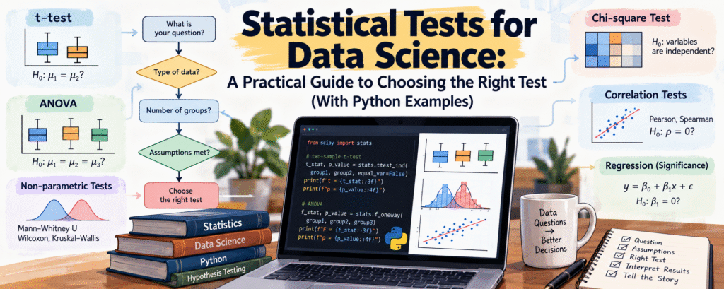
Statistical tests are the rhythm section of data science. Unglamorous, rarely discussed at conferences, but when they drift, the entire set falls apart.
This guide is about picking the right one, reading it correctly, and not embarrassing yourself in a launch review.
Why This Topic Matters
Most DS work reduces to one question: is this difference real, or is it noise?
Confusion matrices and ROC curves get the glory. But the moment you compare two groups — a control and a variant, a model and a baseline, last month and this month — you’re doing hypothesis testing whether you admit it or not.
Get it wrong and you get: false features shipped, dead features killed, drift alarms that cry wolf, and feature selection pipelines that memorize noise.
The transformation this article delivers: you’ll stop treating p < 0.05 as a verdict and start treating it as one input into a decision. You’ll know which test to reach for, which assumptions actually matter, and which ones are academic theater at n = 500,000.
Background: What a Statistical Test Actually Is
Strip away the notation and a test is a weirdness meter.
You posit a boring world — the null hypothesis, H₀. Under H₀, you compute how surprising your observed data would be. If it’s very surprising, you get a small p-value and start doubting the boring world.
That’s it. Fisher introduced the null hypothesis in The Design of Experiments (1935). Neyman and Pearson later bolted on the alternative hypothesis, power, and Type I/II error rates — producing a genuinely two-headed discipline that still argues with itself.
The Fisher vs. Neyman-Pearson Schism
This is the Oasis vs. Blur of statistics, and it never got resolved.
- Fisher: the p-value is a continuous measure of evidence. No magic threshold.
- Neyman-Pearson: it’s a decision rule. Pre-set α, pre-set power, act.
Modern practice Frankenstein-mashed both: a Fisherian p-value judged against a Neyman-Pearson α = 0.05, with post-hoc power calculations that neither man would endorse.
The American Statistical Association finally intervened in 2016 with a statement on p-values, listing six principles. The most important one: a p-value is not a measure of the probability that H₀ is true. It’s P(data this extreme | H₀).
Say that out loud before your next experiment review.
The Two Error Types You Keep Mixing Up
| Reality | You reject H₀ | You fail to reject H₀ |
|---|---|---|
| H₀ true | Type I error (α) | Correct |
| H₀ false | Correct (power = 1−β) | Type II error (β) |
Alpha is the fire alarm that goes off when there’s no fire. Beta is the alarm that stays silent during one. In industry we obsess over alpha and let beta run wild — which is why underpowered tests quietly kill good ideas.
Core Concepts: The Test Selection Decision Tree
Before touching a function, answer three questions:
- What kind of data? Continuous, ordinal, or categorical.
- How many groups? Two, or more than two.
- Are observations independent? Paired/repeated, or independent samples.
Get those three right and 90% of test selection is mechanical.
The Master Comparison Table
| Scenario | Data type | Test | scipy function |
|---|---|---|---|
| 2 groups | continuous, ~normal, equal var | Student’s t | ttest_ind(equal_var=True) |
| 2 groups | continuous, unequal var | Welch’s t | ttest_ind(equal_var=False) |
| 2 groups | skewed / ordinal | Mann-Whitney U | mannwhitneyu |
| Paired | ~normal | Paired t | ttest_rel |
| Paired | skewed / ordinal | Wilcoxon signed-rank | wilcoxon |
| 3+ groups | ~normal | One-way ANOVA | f_oneway |
| 3+ groups | skewed | Kruskal-Wallis | kruskal |
| 3+ repeated | ~normal | RM-ANOVA | statsmodels AnovaRM |
| 3+ repeated | skewed | Friedman | friedmanchisquare |
| 2×2 categorical | small counts | Fisher’s exact | fisher_exact |
| r×c categorical | large counts | Chi-square | chi2_contingency |
| 2 distributions | any | Kolmogorov-Smirnov | ks_2samp |
| Any | exchangeable, weird statistic | Permutation test | permutation_test |
A mistake I see beginners make is defaulting to Student’s t everywhere. In a revenue metric — which is a Gamma-shaped monster with a long tail — that’s the statistical equivalent of playing “Free Bird” at a wedding. Technically a request, practically a disaster.
Welch’s t-test Is the Default, Not the Exception
Student’s t-test assumes equal variances. That’s rarely true in production data, and checking it is a nuisance. Welch’s version drops the assumption:
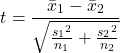
The denominator is the Welch–Satterthwaite approximation to the degrees of freedom, and it costs you almost nothing when variances are equal.
My strong opinion: equal_var=False should be your default in ttest_ind. The power loss is trivial, and you eliminate an entire class of silent errors.
Rank Tests Are Not “Inferior t-tests”
Mann-Whitney U works on ranks. For each pair across both groups, count how often treatment beats control:
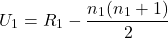
Under H₀ with no ties, U is approximately normal with mean  and variance
  .
.
The key insight most tutorials skip: U tests a different null. It tests stochastic dominance — P(X > Y) = 0.5. If your metric has a heavy tail and you care about mean revenue, Mann-Whitney says “the ranks shifted” while your CFO asks “did revenue move?”
In a deployment I worked on, a rank test flagged a 0.0001 p-value from a promotion that added a few whale purchases. The median user saw nothing. The mean was up 4%. Both statements were true. Only one mattered to the business.
Rank tests are the Cure’s Disintegration: widely respected, misunderstood, and not a substitute for the loud commercial thing you actually wanted.
Chi-Square and Fisher: Categorical Tests
For contingency tables, chi-square measures divergence between observed and expected counts:
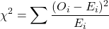
Report Cramér’s V alongside it for effect size:
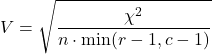
Rule of thumb: chi-square’s approximation degrades when any expected count drops below 5. That’s when you switch to fisher_exact — the exact hypergeometric calculation that Fisher derived (legend says for a lady tasting tea).
I’ve lost count of the number of “significant” segment analyses I’ve seen where 8 of the 40 cells had expected counts under 3. The p-value was fiction.
The Normality Test Trap
A deeper mistake: running Shapiro-Wilk as a gatekeeper for t-tests.
from scipy import stats
# p < 0.05 means "not normal" -- with n=50,000 it always is
print(stats.shapiro(sample))
Large samples reject normality almost always. Tiny samples can’t detect real deviations. The test answers the wrong question.
What you actually care about is whether the sampling distribution of the mean is close enough to normal. That’s the Central Limit Theorem, and with n > ~100 per group it usually bails you out — unless the distribution is genuinely pathological.
Use stats.anderson or normaltest for exploration. Use Q-Q plots visually. Do not use normality tests as binary decision gates.
Effect Size: The Part Everyone Skips
A p-value scales with n. An effect size doesn’t. Cohen’s d:

Conventions: 0.2 small, 0.5 medium, 0.8 large (Cohen, 1988). For non-parametric comparisons, use Cliff’s delta or the rank-biserial correlation instead.
Practical translation: at n = 1,000,000, a d of 0.005 will be “significant.” It will not be worth shipping.
Multiple Comparisons: Spinal Tap’s Amplifier
Run 20 independent tests at α = 0.05 with no true effects and you expect one false positive. Run 10,000 features and you’ll get 500 “discoveries” before breakfast.
Three corrections, in increasing order of reasonableness:
- Bonferroni: test at α/m. Controls family-wise error but is brutally conservative.
- Holm-Bonferroni: step-down version of the same idea, uniformly more powerful.
- Benjamini-Hochberg: controls the false discovery rate — the expected proportion of false positives among your rejections.
BH procedure: sort p-values ascending, find the largest k such that

Reject everything up to k. In high-dimensional feature selection or genomics, BH is the correct tool. Bonferroni is what you use when a single false positive is genuinely catastrophic — say, in a safety-critical medical screen.
Since SciPy 1.11 you can call it directly:
from scipy import stats

p_values = np.array([0.001, 0.008, 0.039, 0.041, 0.09, 0.21, 0.54])
rejected = stats.false_discovery_control(p_values, method="bh")
print(rejected)  # array([0.007, 0.028, 0.0682, 0.0682, 0.09, 0.21, 0.54]) -- BH-adjusted q-values
print(rejected < 0.05)
For Holm and Bonferroni, reach for statsmodels.stats.multitest.multipletests.
Permutation Tests: The Assumption-Light Escape Hatch
If you can compute a test statistic, you can permute. Shuffle group labels thousands of times, recompute the statistic under each shuffle, and see how extreme your observed value is.
from scipy import stats
import numpy as np

rng = np.random.default_rng(7)
observed_diff = treatment.mean() - control.mean()

res = stats.permutation_test(
    (treatment, control),
    lambda x, y: np.mean(x) - np.mean(y),
    n_resamples=10_000,
    alternative="two-sided",
    random_state=rng,
)
print(res.pvalue, res.null_distribution.mean())
Available since SciPy 1.8. It requires exchangeability — valid under random assignment, invalid if your groups are clusters (users in different cities, for example).
During a hyperparameter tuning experiment on a skewed latency metric, a permutation test on the 95th percentile gave me a result the t-test on the mean completely missed. The mean was flat. The tail was not. That changed the entire recommendation.
Practical Applications: Where This Shows Up in Industry
A/B Testing at Scale
Microsoft’s ExP platform, Google, Netflix, and practically every consumer tech firm run controlled experiments as their primary causal inference engine. Kohavi, Longbotham and colleagues documented seven recurring pitfalls in web experiments — most are statistical, not engineering.
The most common one I see: analyzing at the wrong unit. Randomizing by user but testing on pageviews violates independence and inflates your effective sample size. Your p-value is confident and wrong.
Detecting Sample Ratio Mismatch (SRM)
If your 50/50 split delivers 50.4/49.6 on 1.2M users, that’s not noise — that’s a bug. Test it with chi-square.
from scipy import stats
observed = [604_800, 595_200]              # 1.2M total
expected = [600_000, 600_000]
chi2, p, dof, _ = stats.chi2_contingency([observed, expected])
print(f"p = {p:.2e}")   # p ~ 1e-18: your bucketing is broken
SRM is the cheapest high-value test in the entire experimentation stack. Learn it.
Model Drift Monitoring
The Kolmogorov-Smirnov two-sample statistic is the max vertical gap between two empirical CDFs:

from scipy import stats
d, p = stats.ks_2samp(train_scores, prod_scores)
# Monitor D, not just p: p grows with sample size, D is stable
Production catches every week, so p shrinks toward zero for even invisible shifts. Monitor D as your drift magnitude, and use p only as a tiebreaker.
Feature Selection in scikit-learn
SelectKBest with f_classif runs an ANOVA F-test per feature and keeps the top k. That’s thousands of hypothesis tests.
from sklearn.feature_selection import SelectKBest, f_classif, chi2, mutual_info_classif

sel = SelectKBest(f_classif, k=200).fit(X_train, y_train)
f_scores, p_values = sel.scores_, sel.pvalues_
Nobody in the tutorial mentions the multiple comparisons problem. If you’re selecting features to interpret, apply BH correction to p_values first. If you’re selecting features purely for predictive power, use mutual_info_classif or model-based selection instead — the F-test’s linearity assumption will quietly hurt you.
Implementation Example: A Complete Comparison Pipeline
Here’s a reusable workflow. It runs three tests, computes effect size, and produces a bootstrap confidence interval.
import numpy as np
from scipy import stats

rng = np.random.default_rng(42)

# Heavy right tail -- the realistic shape of revenue-per-user data
control   = rng.gamma(shape=2.0, scale=1.00, size=20_000)
treatment = rng.gamma(shape=2.0, scale=1.05, size=20_000)   # ~5% mean lift

# ---------- 1. Parametric ----------
t, p_welch = stats.ttest_ind(treatment, control, equal_var=False)
print(f"Welch t-test        : t = {t:7.3f}   p = {p_welch:.5f}")

# ---------- 2. Non-parametric ----------
u, p_mwu = stats.mannwhitneyu(treatment, control, alternative="two-sided")
print(f"Mann-Whitney U      : U = {u:9.1f}  p = {p_mwu:.5f}")

# ---------- 3. Assumption-light ----------
perm = stats.permutation_test(
    (treatment, control),
    lambda x, y: np.mean(x) - np.mean(y),
    n_resamples=10_000,
    alternative="two-sided",
    random_state=rng,
)
print(f"Permutation (mean)  : p = {perm.pvalue:.5f}")

# ---------- 4. Effect size ----------
def cohens_d(a, b):
    n1, n2 = a.size, b.size
    s = np.sqrt(((n1 - 1) * a.var(ddof=1) + (n2 - 1) * b.var(ddof=1)) / (n1 + n2 - 2))
    return (b.mean() - a.mean()) / s

print(f"Cohen's d           : {cohens_d(control, treatment):.4f}")
print(f"Relative lift       : {treatment.mean() / control.mean() - 1:.2%}")

# ---------- 5. Bootstrap CI on the relative lift ----------
boot = np.array([
    rng.choice(treatment, treatment.size, replace=True).mean()
    / rng.choice(control, control.size, replace=True).mean() - 1
    for _ in range(5_000)
])
lo, hi = np.percentile(boot, [2.5, 97.5])
print(f"95% bootstrap CI    : [{lo:.2%}, {hi:.2%}]")
How to read the output. If Welch says p = 0.03, Mann-Whitney says p = 0.001, and the bootstrap CI is [0.4%, 9.6%], you have a real but uncertain shift. Your call depends entirely on whether a 0.4% lift covers the engineering cost.
Note the CI width is what actually drives the decision. A CI that spans zero plus a CI that spans 0.1% are different conversations.
Debugging, Pitfalls, and Strong Opinions
Peeking at your experiment. Sequential testing without alpha-spending inflates Type I error. Use sequential tests (always-valid inference, group sequential boundaries) or fix the horizon. This is why I use statsmodels group-sequential methods rather than eyeballing a daily dashboard.
Treating “not significant” as “no effect.” Absence of evidence is not evidence of absence. Report the CI. If it spans both a harmful and a beneficial effect, your experiment was underpowered — say so.
Assuming independence in clustered data. Users in the same household, sessions from the same device, samples from the same batch. Use cluster-robust methods or mixed-effects models.
Simpson’s paradox. Aggregate can flip sign versus every subgroup. Always segment before believing an aggregate win.
The “we’ll just use a t-test” reflex on skewed metrics. Million-user samples make the CLT tolerable for means, but percentiles and ratios are not means. Use the delta method or bootstrap.
Post-hoc power analysis. Computing power after seeing your p-value is circular. Power is a design-time quantity.
Forgetting that the p-value doesn’t rank effect sizes. A tiny study can produce p = 0.049 with d = 2.0, and a giant study p = 0.001 with d = 0.01. Never compare significance across studies. Compare effects.
Ignoring SRM and guardrail metrics. Your primary metric can win while latency, crash rate, or retention silently degrade. Guardrails use the same test machinery — so use it.
Using the wrong tail. alternative="two-sided" unless you pre-registered a direction. One-sided tests chosen after looking at the data are p-hacking with a lab coat on.
Future Outlook
Three shifts are already underway.
Bayesian A/B testing. Frameworks like PyMC and Google’s abracadabra report the probability that variant B beats A, which is what stakeholders actually want. You trade frequentist error guarantees for decision-relevant probabilities. Not a free lunch — just a different lunch.
Variance reduction. CUPED (controlled-experiment using pre-experiment data), stratified sampling, and regression adjustment routinely cut required sample sizes by 30–50%. Netflix and Microsoft publish on this. It’s less a statistical test than an efficiency multiplier for the tests you already run.
Continuous monitoring and adaptive designs. Always-valid p-values, group sequential boundaries, and multi-armed bandits replace the fixed-horizon test as the default in high-velocity product teams.
Philosophically, there’s something conservative worth saying here. The whole hypothesis-testing apparatus exists because humans are pattern-matching machines that see faces in clouds. The p-value, for all its flaws, is a discipline against our own enthusiasm. It’s the studio engineer insisting you play to a click track.
You can hate the click track. You should still use it.
Summary: Key Takeaways
- A p-value answers P(data this extreme | H₀). It never answers P(H₀ | data), and it never measures importance.
- Welch’s t-test over Student’s as your default. The equal-variance assumption earns nothing and costs accuracy.
- Effect size and confidence intervals outrank p-values for decisions. A significant 0.02% lift is a rounding error with a strong resume.
- Rank tests test a different null. Use them for ordinal or tail-dominated metrics, but understand what claim you’re buying.
- Correct for multiple comparisons — BH for discovery, Bonferroni/Holm for safety. Never skip this in feature selection or segment analysis.
- Permutation tests are the assumption-light fallback whenever exchangeability holds and the statistic is computable.
The sticky metaphor: statistical tests are the rhythm section. The t-test is your bassist — reliable, slightly boring, plays the root. The Mann-Whitney U is a displaced jazz drummer, technically dazzling and testing something slightly different than you thought. Bonferroni is the metronome that won’t let anyone go to 11. And the p-value is the click track: nobody notices it when it’s right, and everything collapses when it isn’t.
Actionable Next Steps
Runnable mini-projects
- Reproduce the simulation above with
shape=1.5(heavy tail) and compare Welch vs. Mann-Whitney vs. permutation across 1,000 simulated runs. Count how often each rejects. You’ll learn more in 30 minutes than in a semester. - Build an SRM detector. Write a function taking a dict of variant → count and returning a chi-square p-value plus a verdict.
- False discovery demo. Generate 10,000 null feature columns and one real one. Run
f_classifand watch 500 fake features light up. Then apply BH and watch them vanish.
Datasets to try
sklearn.datasets.load_breast_cancerfor feature selection with FDR correction.- UCI Online Retail II for skewed revenue metrics and permutation testing.
- Any public A/B dataset from Kaggle — but check the assignment mechanism before trusting it.
References & Further Reading
Foundational papers and statements
- Wasserstein, R. L., & Lazar, N. A. (2016). The ASA Statement on p-Values: Context, Process, and Purpose. The American Statistician, 70(2), 129–133.
- Wasserstein, R. L., Schirm, A. L., & Lazar, N. A. (2019). Moving to a World Beyond “p < 0.05”. The American Statistician, 73(S1).
- Benjamini, Y., & Hochberg, Y. (1995). Controlling the False Discovery Rate: A Practical and Powerful Approach to Multiple Testing. JRSS-B, 57(1), 289–300.
- Cohen, J. (1988). Statistical Power Analysis for the Behavioral Sciences (2nd ed.). Lawrence Erlbaum.
- Kohavi, R., Crook, T., & Longbotham, R. (2009). Online Experimentation at Microsoft. Third Workshop on Data Mining Case Studies.
- Crook, T., Frasca, B., Kohavi, R., & Longbotham, R. (2009). Seven Pitfalls to Avoid When Running Controlled Experiments on the Web. KDD ’09.
- Deng, A., Xu, Y., Kohavi, R., & Walker, T. (2013). Improving the Sensitivity of Online Controlled Experiments by Utilizing Pre-Experiment Data (CUPED). WSDM ’13.
- Fisher, R. A. (1935). The Design of Experiments. Oliver & Boyd.
Documentation
- SciPy
statsmodule: hypothesis tests and statistical functions — https://docs.scipy.org/doc/scipy/reference/stats.html scipy.stats.permutation_test(added 1.8.0) — https://docs.scipy.org/doc/scipy/reference/generated/scipy.stats.permutation_test.htmlscipy.stats.false_discovery_control(added 1.11.0) — https://docs.scipy.org/doc/scipy/reference/generated/scipy.stats.falsediscoverycontrol.html- scikit-learn feature selection — https://scikit-learn.org/stable/modules/feature_selection.html
- statsmodels multiple testing (
multipletests) — https://www.statsmodels.org/stable/generated/statsmodels.stats.multitest.multipletests.html - PyMC for Bayesian A/B testing — https://www.pymc.io/
Books worth owning
- Kohavi, R., Tang, D., & Xu, Y. (2020). Trustworthy Online Controlled Experiments. Cambridge University Press.
- Efron, B., & Tibshirani, R. J. (1993). An Introduction to the Bootstrap. Chapman & Hall.
- Gelman, A., Carlin, J. B., Stern, H. S., et al. (2013). Bayesian Data Analysis (3rd ed.). CRC Press.
Related posts:
 The Statistical Mind: How Mastering Data’s Language Can Save You From Digital Deception
 The Unseen Architects of Reality: How Discrete Probability Distributions Govern Your Digital World
 The Unseen Architects of Reality: Mastering Continuous Probability Distributions for Data Dominance
 Data science interview preparation kit
Leave a Reply