
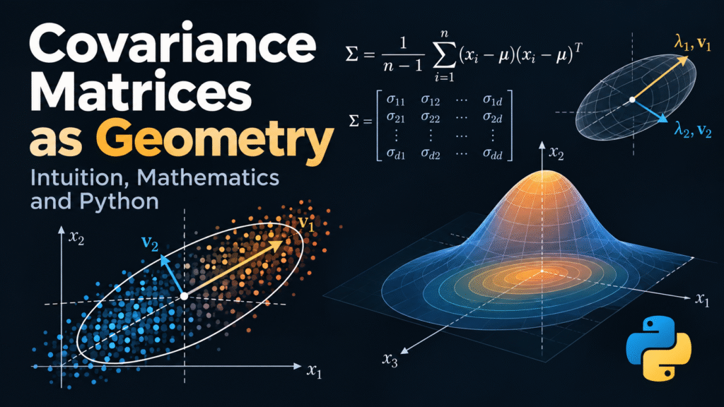
Most people meet the covariance matrix as a table. A spreadsheet of variances on the diagonal and covariances off it, produced by np.cov, printed in a notebook, never looked at again. That is a shame, because the covariance matrix is not really a table. It is a shape. It is a description of how a cloud of points is stretched, rotated and tilted in space — and once you read it as geometry, a dozen techniques (PCA, whitening, Mahalanobis distance, Cholesky sampling, Gaussian graphical models) stop being separate tricks and become the same idea wearing different hats.
Consider two datasets. Both have two features, both standardized to unit variance. One is a round cloud. The other is a diagonal streak.
import numpy as np

rng = np.random.default_rng(0)
n = 500

z = rng.standard_normal((2, n))          # round cloud

A = np.array([[1.0, 0.0],
              [0.9, 0.44]])
x = A @ z                                # shear: feature 2 tracks feature 1

print(np.cov(z))   # ~ identity
print(np.cov(x))   # same diagonal, large off-diagonal
Marginal variances of x are 1.0 and 1.0036 in expectation. Identical spread per feature. And yet the two datasets are not remotely the same object, and any algorithm that treats features independently — naive Bayes, L2 distance, a diagonal-covariance Gaussian — sees them as identical. The diagonal of the covariance matrix threw away the only information that mattered.
That gap between “how much each feature varies” and “what shape the data has” is the subject of this article.
Why This Matters
The covariance matrix is, arguably, the most load-bearing object in classical multivariate statistics and a great deal of machine learning. A partial list of places it is quietly doing the work:
- Dimensionality reduction. PCA is nothing more than the eigendecomposition of a covariance (or correlation) matrix. The principal directions are its eigenvectors; the explained variance is its eigenvalues.
- Distance and anomaly detection. The Mahalanobis distance is Euclidean distance measured in the geometry the covariance matrix defines. It is the backbone of multivariate outlier detection, Gaussian discriminant analysis and many fraud models.
- Whitening and preconditioning. Many optimizers and models behave far better when inputs are decorrelated and rescaled. Whitening is a linear change of coordinates defined by Σ.
- Sampling and simulation. To draw from a multivariate Gaussian, you factor Σ = LLᵀ (Cholesky) and multiply standard normal draws by L. The geometry of Σ is the geometry of the sampler.
- Regression with correlated errors. Generalized least squares uses Σ^{-1} as a metric to weight observations correctly. Ignoring it is how you get confidently wrong standard errors.
- Gaussian processes and Kalman filters. Both are, at their core, bookkeeping systems for covariance matrices — and the numerical difficulties they hit are covariance-matrix difficulties.
- Conditional independence. The inverse covariance (precision matrix) encodes which variables are independent given all the others, which is the basis of Gaussian graphical models and graphical lasso.
When this object is misunderstood, the failure modes are quiet and expensive. A PCA on unstandardized features does not crash; it silently reports a component that is just whichever feature happened to be measured in millimeters. A Mahalanobis distance computed with a singular sample covariance does not crash; it returns a number with enormous variance driven by numerical noise.
By the end, you should be able to explain why Σ is best understood as a linear operator and a metric, derive the ellipse interpretation from the spectral theorem, implement the whole pipeline from scratch in NumPy, and know exactly when the geometry you extracted is a lie.
Prerequisites
- Vectors, matrices, matrix multiplication, inner products.
- Expectation, variance, covariance of random variables.
- Basic Python and NumPy.
- Helpful but not required: Eigenvalues and Eigenvectors, Probability Distributions.
Intuition: The Matrix Is an Ellipse
Here is the single most useful mental model. Take a cloud of points. Center it. Draw the smallest ellipse that captures its shape. That ellipse has:
- directions (which way it is tilted),
- lengths (how far it extends along each direction).
The covariance matrix stores exactly those two things, plus nothing else. Its eigenvectors are the ellipse’s axes. The square roots of its eigenvalues are the semi-axis lengths.
Why “nothing else”? Because covariance is a second-moment summary. It is the linear part of the description. It knows about spread and tilt. It knows nothing about whether the cloud is a single blob, a crescent, or two separate blobs.
Two equivalent ways to see the same object:
Σ as a linear map. Σ is a d × d matrix, so it is a function from ℝᵈ to ℝᵈ. It acts by stretching every vector along the eigenvector directions, by factors λ₁, …, λ_d. Push the unit sphere through this map and you get an ellipsoid. The covariance matrix is the machine that turns a circle into the ellipse.
Σ as a metric. A metric is a rule for measuring lengths. Σ^{-1} redefines “how far apart are these two points” so that one standard deviation in the short direction of the ellipse counts the same as one standard deviation in the long direction. That is the Mahalanobis distance. Whitening is just the coordinate change that turns this odd metric back into ordinary Euclidean distance.
Both views are the same statement in different clothing: the eigenvectors are the axes, and the eigenvalues tell you how the axes are scaled.
A concrete numeric example is worth more than a paragraph. Take
import numpy as np
from numpy.linalg import eigh

Sigma = np.array([[2.0, 0.8],
                  [0.8, 0.5]])

vals, vecs = eigh(Sigma)                 # ascending
order = np.argsort(vals)[::-1]
vals, vecs = vals[order], vecs[:, order]

print("eigenvalues:      ", vals)        # [2.3466  0.1534]
print("semi-axis lengths:", np.sqrt(vals))
print("axis directions:  ", vecs[:, 0])  # ~ [0.918 0.397]
print("trace:", vals.sum(), " det:", vals.prod())
The eigenvalues are ≈ 2.347 and ≈ 0.153, summing to the trace 2.5 and multiplying to the determinant 0.36. The major axis points in direction ≈ (0.918, 0.397), about 23 degrees above the horizontal. In one eigendecomposition you have recovered the total variance, the “volume” of the ellipse, its orientation and its elongation. The ratio λ₁/λ₂ ≈ 15.3 says the cloud is 15 times longer than it is wide — a fact invisible in the diagonal entries 2.0 and 0.5 alone.
Mathematical Foundation
Definition
Let X ∈ ℝᵈ be a random vector with mean μ = 𝔼[X]. The covariance matrix is
Σ = 𝔼[(X − μ)(X − μ)ᵀ].
Entry (i, j) is Cov(Xᵢ, Xⱼ), and by symmetry of covariance, Σ = Σᵀ. Because (X − μ)(X − μ)ᵀ is an outer product, Σ is a sum of outer products — which is the structural reason it is positive semidefinite.
Why Σ Is Positive Semidefinite
For any a ∈ ℝᵈ,
aᵀΣa = 𝔼[aᵀ(X − μ)(X − μ)ᵀa] = 𝔼[(aᵀ(X − μ))²] = Var(aᵀX) ≥ 0.
This is not a technicality; it is the geometric heart of the matter. A vector a defines a one-dimensional projection of your data. Its variance is aᵀΣa. So the covariance matrix is a machine that answers the question “how much variance is there in direction a?” for every direction simultaneously. Positivity is just the statement that variance cannot be negative.
There is a second reading worth keeping. Variance is an inner product on the space of centered random variables: ⟨Y, Z⟩ = 𝔼[YZ]. Under that inner product, Σ is precisely the Gram matrix of the centered coordinates X₁ − μ₁, …, Xd − μd. That is why the PSD proof is one line: it is Cauchy–Schwarz in disguise. It also explains why covariance is fundamentally about inner products, which is why it plays nice with kernels and Gram matrices later.
Spectral Theorem and the Ellipse
Since Σ is symmetric, the spectral theorem gives
Σ = Q Λ Qᵀ, Q orthogonal (QᵀQ = I), Λ = diag(λ₁ ≥ λ₂ ≥ … ≥ λ_d ≥ 0).
Columns of Q are the eigenvectors; eigenvalues are non-negative. The consequence is the ellipse.
Let T = Σ^{1/2} = Q Λ^{1/2} Qᵀ. If u ranges over the unit sphere, Tu traces out the ellipsoid. A unit vector aligned with q₁ gets stretched to length √λ₁; aligned with qd, to length √λd. So the ellipsoid has semi-axes √λᵢ qᵢ. Because det T = ∏√λᵢ = (det Σ)^{1/2}, and because T maps the unit ball to the ellipsoid, the volume is scaled by exactly that factor:
Vol(ellipsoid) = Vd · √(det Σ), where Vd = π^{d/2} / Γ(d/2 + 1).
Two identities follow immediately and are worth memorizing:
- trace(Σ) = Σλᵢ = total variance. Adding up all the per-feature variances equals adding up the eigenvalues.
- det(Σ) = ∏λᵢ = “generalized variance”. It is proportional to the squared volume of the ellipsoid. If det(Σ) = 0, the ellipsoid is flat — the data live in a lower-dimensional subspace.
Which Matrix Has the Ellipse — Σ or Σ^{-1}?
This trips up nearly everyone at least once. Both Σ and Σ^{-1} have the same eigenvectors, since Σ^{-1} = Q Λ^{-1} Qᵀ. But the level sets differ in meaning:
- {x : xᵀΣ^{-1}x = c} is an ellipse whose semi-axes have lengths √(c λᵢ). This is the constant-density contour of a Gaussian, because the density is ∝ exp(−½ xᵀΣ^{-1}x).
- {x : xᵀΣx = c} is an ellipse whose semi-axes have lengths √(c / λᵢ) — the reciprocal lengths, because the eigenvalues of Σ^{-1} are 1/λᵢ.
Rule of thumb: Σ^{-1} draws the contours of the distribution; Σ describes the shape of the map. When a density plot looks wrong, check which one you used.
Mahalanobis Distance Is Whitened Euclidean Distance
Define the Mahalanobis distance
D_M(x, μ)² = (x − μ)ᵀ Σ^{-1} (x − μ).
Now define the transformation z = Σ^{-1/2}(x − μ). Then
‖z‖² = (x − μ)ᵀ Σ^{-1/2} Σ^{-1/2} (x − μ) = D_M(x, μ)²,
and moreover
Var(z) = Σ^{-1/2} Σ Σ^{-1/2} = I.
So the Mahalanobis distance is ordinary Euclidean distance computed in a coordinate system where the cloud is a perfect unit sphere. The two operations — measuring distance properly and whitening the data — are literally the same operation viewed from opposite ends. This is why z-scores are the one-dimensional special case: with Σ = diag(σ₁², …, σ_d²), the Mahalanobis distance reduces to the sum of squared z-scores.
For a d-dimensional Gaussian, the squared Mahalanobis distance of a sample follows a chi-squared distribution with d degrees of freedom. Its mean is d. That single fact underpins a large fraction of practical multivariate outlier detection.
PCA Falls Out of a One-Line Optimization
Suppose we want the direction w (unit norm) with the largest variance of the projection wᵀX. We are maximizing
maximize wᵀΣw subject to wᵀw = 1.
The Lagrangian is L(w, λ) = wᵀΣw − λ(wᵀw − 1). Setting ∂L/∂w = 2Σw − 2λw = 0 gives
Σw = λw.
The optimal direction is an eigenvector, and the achieved variance is wᵀΣw = λwᵀw = λ. Therefore the maximum-variance direction is the top eigenvector, with variance λ₁. Constraining subsequent components to be orthogonal to the previous ones gives the remaining eigenvectors in order. That is PCA, derived in four lines, and it is the same ellipse from before.
The general statement is the Rayleigh quotient: for any nonzero w,
λmin ≤ (wᵀΣw)/(wᵀw) ≤ λmax.
Every projection of your data has variance somewhere between the smallest and largest eigenvalue. This is why PCA truncation is meaningful: discarding the small eigenvalues discards directions where there is almost nothing to see.
Where the Sample Matrix Comes From (and Why n − 1)
For i.i.d. Gaussian data x₁, …, x_n, the negative log-likelihood is
−ℓ(μ, Σ) = (n/2) log det Σ + ½ Σᵢ (xᵢ − μ)ᵀ Σ^{-1} (xᵢ − μ) + const.
Differentiating with respect to μ gives μ̂ = x̄. Differentiating with respect to Σ, using ∂ log det Σ / ∂Σ = Σ^{-1}, gives the maximum likelihood estimate
Σ̂_MLE = (1/n) Σᵢ (xᵢ − x̄)(xᵢ − x̄)ᵀ = ((n−1)/n) · S, where S = (1/(n−1)) Σᵢ (xᵢ − x̄)(xᵢ − x̄)ᵀ.
Since 𝔼[Σᵢ (xᵢ − x̄)(xᵢ − x̄)ᵀ] = (n−1)Σ, the MLE is biased low by the factor (n−1)/n, and the unbiased estimator is S — which is what np.cov returns by default. The bias is a degrees-of-freedom effect: you spent one degree of freedom estimating the mean. For large n it is irrelevant; for n = 5 it is a 20% understatement of variance.
This is the likelihood → log-likelihood → estimator chain that also produces logistic regression and, well, most of statistics. The same likelihood appears in Gaussian discriminant analysis, where classes differ only in μ, and the shared Σ is estimated by pooling within-class scatter: Σ̂w = Σc (nc/n) Sc. Invert it and you have Fisher’s linear discriminant direction, w ∝ Σ̂w^{-1}(μ̂₁ − μ̂₀). The geometry of Σ̂w^{-1} determines which direction best separates the classes — that is, which direction has the most signal relative to the noise ellipse.
A Brief Note on Fisher Information
One more structural fact, because it connects statistics to differential geometry. For a parametric model p(x; θ), the Fisher information matrix is
I(θ) = 𝔼[∇θ log p(x; θ) (∇θ log p(x; θ))ᵀ],
which is a covariance matrix of the score vector, and therefore symmetric PSD. It defines a Riemannian metric on the parameter space (the Fisher–Rao metric), and its inverse bounds the variance of any unbiased estimator via the Cramér–Rao inequality. In other words, the same PSD geometry shows up on the parameter side, not just the data side. That is not a coincidence; it is a signature of information geometry, and it is why natural gradient methods precondition by I(θ).
From Mathematics to Data Science
The conceptual chains, stated plainly:
- Inner product → Gram matrix → sample covariance → eigendecomposition → PCA → dimensionality reduction.
- Covariance → metric Σ^{-1} → Mahalanobis distance → outlier detection, anomaly scoring, Gaussian discriminant analysis.
- Covariance → factorization Σ = LLᵀ → correlated sampling → Monte Carlo, Gaussian processes, Kalman filters.
- Covariance → inverse → partial correlations → Gaussian graphical models → conditional independence structure.
- Covariance → Cholesky/whitening → preconditioning → faster and more stable optimization.
- Covariance → correlation matrix (covariance of standardized data) → scale-invariant analysis.
And a chain that connects the two views of this article: the linear map view and the metric view are related by inversion. Σ tells you the shape; Σ^{-1} tells you the price of distance. Everything downstream of covariance is a choice about whether you need the shape or the price.
Python Implementation (From Scratch)
Two datasets below: one generated from the Cholesky factor of a known Σ, which is also the cleanest way to produce correlated data.
import numpy as np
import matplotlib.pyplot as plt
from matplotlib.patches import Ellipse

rng = np.random.default_rng(7)

# ---------- 1. Build a cloud with a known geometry ----------
Sigma_true = np.array([[2.0, 0.8],
                       [0.8, 0.5]])

L = np.linalg.cholesky(Sigma_true)      # Sigma = L @ L.T
Z = rng.standard_normal((2, 5000))      # unit-variance round cloud
X = L @ Z                               # shear + stretch

print("Cholesky factor:\n", L)
print("Sample covariance:\n", np.cov(X))

# ---------- 2. Read the geometry out of the matrix ----------
S = np.cov(X)                           # unbiased, rows are variables
vals, vecs = np.linalg.eigh(S)          # symmetric eigensolver
idx = np.argsort(vals)[::-1]
vals, vecs = vals[idx], vecs[:, idx]

print("eigenvalues:  ", vals)
print("semi-axes:    ", np.sqrt(vals))
print("major axis dir:", vecs[:, 0])
print("angle (deg):  ", np.degrees(np.arctan2(vecs[1, 0], vecs[0, 0])))
print("trace = total variance:", vals.sum(), "| det = generalized variance:", np.prod(vals))

# ---------- 3. Whitening: the ellipse becomes a circle ----------
W = np.linalg.inv(L)                    # equals S^{-1/2} up to sampling error
Xw = W @ (X - X.mean(axis=1, keepdims=True))
print("Whitened covariance (should be ~I):\n", np.cov(Xw))

# ---------- 4. Mahalanobis distance via Cholesky, not inversion ----------
def mahalanobis_sq(X, mu, Sigma):
    d = X - mu[:, None]
    Lc = np.linalg.cholesky(Sigma)
    y = np.linalg.solve(Lc, d)          # triangular solve
    return np.sum(y**2, axis=0)

md2 = mahalanobis_sq(X, X.mean(axis=1), S)
print("mean squared Mahalanobis distance (theory: 2):", md2.mean())

# ---------- 5. Draw it ----------
fig, ax = plt.subplots(figsize=(5, 5))
ax.scatter(X[0], X[1], s=4, alpha=0.25)

angle = np.degrees(np.arctan2(vecs[1, 0], vecs[0, 0]))
for k in (1, 2):
    e = Ellipse(xy=X.mean(axis=1),
                width=2 * k * np.sqrt(vals[0]),
                height=2 * k * np.sqrt(vals[1]),
                angle=angle, fill=False)
    ax.add_patch(e)

ax.set_aspect("equal")
ax.set_title("Data cloud with 1- and 2-sigma ellipses")
plt.show()
A few things to note in that code, because each one is a habit worth forming:
- Use
eigh, noteig.eightargets symmetric matrices, returns real eigenvalues, and is faster and more accurate. - Sort eigenvalues yourself.
eighreturns them ascending; descending order is the convention because component 1 should be the most important. - Solve, don’t invert.
np.linalg.solve(L, d)with the Cholesky factor is cheaper and more numerically stable than forminginv(Sigma)and multiplying. - Cholesky requires positive definiteness. If it raises a
LinAlgError, your matrix is singular or your data are numerically rank-deficient — which is a diagnosis, not an inconvenience.
The mean squared Mahalanobis distance should print close to 2.0, because for a d = 2 Gaussian the squared Mahalanobis distance is χ²₂ with mean 2. That is a one-line sanity check on the entire geometry.
The Library Version
from sklearn.covariance import EmpiricalCovariance, LedoitWolf, MinCovDet
from sklearn.decomposition import PCA

Xr = X.T                                  # sklearn wants (n_samples, n_features)

pca = PCA(n_components=2).fit(Xr)
print("explained variance:", pca.explained_variance_)
print("components:\n", pca.components_)

emp = EmpiricalCovariance().fit(Xr)
print("Mahalanobis (sklearn):", emp.mahalanobis(Xr[:5]).round(3))

lw = LedoitWolf().fit(Xr)
mcd = MinCovDet(random_state=0).fit(Xr)
print("shrinkage of Ledoit-Wolf:", lw.shrinkage_)
The relationship is exact, not approximate. PCA computes the eigendecomposition of the covariance (or correlation) matrix; pca.explained_variance_ is the eigenvalue vector, and pca.components_ are the eigenvectors. EmpiricalCovariance().mahalanobis() computes exactly the mahalanobis_sq above. The library adds regularization options (LedoitWolf for shrinkage, MinCovDet for robust estimation) and API polish, not a different mathematics. If you can write the from-scratch version, reading the library’s source is mostly bookkeeping.
Computational Experiment: When Does a Sample Covariance Matrix Start Lying?
This is the question that separates textbook covariance from production covariance.
Hypothesis
For i.i.d. standard normal data in d dimensions with n samples, the sample covariance matrix is a good estimate of the identity when d ≪ n, and a wildly misleading one when d is comparable to n. Even with zero real structure, the eigenvalues of the sample covariance spectrum will spread out, and PCA will “discover” components.
The theoretical anchor is the Marchenko–Pastur law: for n, d → ∞ with d/n → γ, the empirical spectrum of the sample covariance of standard normal data converges to a density supported on
[(1 − √γ)², (1 + √γ)²], with mean 1.
At γ = 1, that support is [0, 4]. The largest sample eigenvalue is around 4 for pure noise. The condition number of the sample covariance is roughly ((1+√γ)/(1−√γ))², which diverges as γ → 1.
Method
Sample standard normal data at several values of γ = d/n, compute the eigenvalues of the sample covariance, and compare the empirical extremes with the theoretical Marchenko–Pastur edges.
Code
import numpy as np

rng = np.random.default_rng(0)
n = 400

print(f"{'gamma':>6} {'theor.lo':>9} {'theor.hi':>9} {'emp.lo':>9} {'emp.hi':>9}")
for gamma in [0.1, 0.4, 0.7, 1.0]:
    d = int(gamma * n)
    X = rng.standard_normal((n, d))          # pure noise, no structure
    S = np.cov(X, rowvar=False)
    eigs = np.linalg.eigvalsh(S)
    lo, hi = (1 - np.sqrt(gamma))**2, (1 + np.sqrt(gamma))**2
    print(f"{gamma:6.1f} {lo:9.2f} {hi:9.2f} {eigs.min():9.2f} {eigs.max():9.2f}")

# Square case: n = d, so the sample covariance is exactly singular
n = d = 400
X = rng.standard_normal((n, d))
Xc = X - X.mean(axis=0)
print("rank of centered data:", np.linalg.matrix_rank(Xc), "of", d)
print("det of sample covariance:", np.linalg.det(np.cov(X, rowvar=False)))

eigs = np.linalg.eigvalsh(np.cov(X, rowvar=False))
print("share of total variance in PC1:", eigs.max() / eigs.sum())
Expected Result
At γ = 0.1 the empirical extremes should sit comfortably inside the theoretical interval [0.47, 1.73]; at γ = 1 they should approach the interval [0, 4] as d grows. In the square case, the centered data matrix has rank n − 1 = 399 while d = 400, so det of the sample covariance is numerically zero (it may come out as a tiny signed number such as 1e-300 or as a small negative value from floating point, not exactly 0), and the condition number is effectively infinite. The first principal component of pure noise captures a share of total variance of order 1/d — small in percentage terms, but far larger than an honest scree plot of real structure would suggest at the tail.
Run it and you will notice the pattern that makes this experiment worth writing down: the spread of the spectrum is a function of d/n, not of any real signal.
Interpretation
The sample covariance is an estimator, and like any estimator it has variance. Here the variance is structured: every feature contributes a little noise to every entry, and the accumulation across d features pushes the extreme eigenvalues away from 1. At γ → 1 the smallest sample eigenvalue collapses toward zero, which means Σ̂^{-1} has an enormous eigenvalue in that direction. Any Mahalanobis distance, whitening transform or discriminant direction that relies on Σ̂^{-1} will then amplify pure sampling noise into a “signal.”
This is the mathematical reason behind a rule practitioners state informally as “don’t trust PCA when you have fewer samples than features.” The rule is correct, and now it has a shape and a scale.
Assumptions
Second-moment geometry is a package deal. Here is what you are buying.
- Finite variance. Covariance exists only if second moments do. For Pareto-like distributions with tail index α ≤ 2, the sample covariance is not a stable estimate and can jump wildly as n grows. Violation is not just theoretical; financial and network data routinely live here.
- The mean is correctly specified. Covariance measures spread around μ. If the true structure is a mixture, the single global mean is the wrong center, and Σ is inflated by the between-component variation.
- Linearity. Σ captures linear dependence only. For the relationship Y = X² with X symmetric, Cov(X, Y) = 0 despite Y being a deterministic function of X.
- Exchangeability / stationarity (for time series). The sample covariance pools all time points. If the process drifts, Σ̂ averages over regimes and describes none of them.
- I.I.D. sampling, for the distributional results. The Wishart distribution of Σ̂, the chi-squared Mahalanobis law and the Marchenko–Pastur limit all assume independent samples from one distribution. Autocorrelation effectively shrinks your sample size, sometimes drastically.
- Gaussianity, specifically for the strong claims. Zero covariance implies independence only for jointly Gaussian variables. For the marginal check “is the covariance spectrum informative?”, heavy tails distort everything.
Mild violations are often survivable. Missing normality usually is: covariances remain meaningful summaries, and many results degrade gracefully. Missing finite variance or stationarity is not survivable in the same way — those need different tools.
Pitfalls and Failure Modes
Mathematical Misconceptions
“Covariance zero implies independence.” False in general. True for jointly Gaussian variables. This single exception is why Gaussian models can get away with using only first and second moments, and why they fail so badly when the data are not Gaussian — a Gaussian model has no vocabulary for a nonlinear dependency.
Confusing Σ with Σ^{-1} in plotting and distance code. As shown above, they share eigenvectors but not eigenvalues. Contours of the density use Σ^{-1}; the shape map uses Σ.
Treating eigenvectors as uniquely identified. Eigenvector signs are arbitrary (v and −v are both valid), and when two eigenvalues are nearly equal, the eigenvectors are not stable at all. The Davis–Kahan theorem bounds the rotation of an eigenvector subspace by ‖E‖ / gap, where E is the perturbation and gap is the separation between eigenvalues. Small gap, unstable direction. If your PCA loadings flip sign between two runs on slightly different data, this is why.
Thinking covariance measures “correlation strength” in a scale-free way. It does not. Covariance has units — the product of the two features’ units. Comparing covariances across feature pairs with different scales is meaningless.
Implementation Mistakes
- Forgetting to center.
np.covcenters by default; hand-rolledX @ X.T / ndoes not, and produces a matrix dominated by the mean. - Wrong orientation for
np.cov. Rows are variables by default. For an (nsamples, nfeatures) array you needrowvar=False. Getting this wrong silently produces an n × n matrix instead of d × d, and with n > d the bug is invisible until something downstream breaks. - Computing PCA on unstandardized features. A feature measured in millimeters will dominate everything. Use the correlation matrix (or standardize first) unless the units are genuinely comparable — and be aware that standardizing to unit variance is itself a modeling choice that amplifies noisy low-variance features.
- Using
eigon a symmetric matrix. You get complex eigenvalues with tiny imaginary parts that break downstream comparisons. - Inverting a covariance matrix. Use
solveor Cholesky. Explicit inversion is slower, less accurate, and squares the condition number. - Preprocessing leakage. Fitting the covariance-based scaler or PCA on the full dataset and then splitting into train/test leaks test information into the training geometry. Fit inside the pipeline.
Statistical Mistakes
- Estimating a d × d covariance from n < d samples. The result is always singular and always overfit to the noise. There is no exception.
- Assuming independence from a covariance matrix computed on pooled groups. Simpson’s paradox has a multivariate version: within-group correlations can have the opposite sign to the pooled correlation.
- Reading causal claims from structure. A covariance matrix tells you what co-moves. It knows nothing about intervention. Sleep and coffee consumption covary enormously and each affects the other; the matrix is silent on which.
Production Failure Modes
- Outliers. The sample covariance has a breakdown point of zero: a single sufficiently extreme point can move entries arbitrarily and rotate eigenvectors by an arbitrary amount. This is not an edge case; in anomaly detection, the anomalies are exactly the points that break your covariance estimate.
- Conditioning. The relative condition number of the covariance is the square of that of the data matrix. Whitening squares it again in the opposite direction. In high dimensions the smallest eigenvalues are dominated by sampling noise, and Σ̂^{-1} blows that noise up.
- Drift. A covariance matrix fitted on 12 months of data describes the average geometry of 12 months. If the geometry changes with the season or with a policy change, you are reweighting today’s data with last year’s metric.
- Reproducibility. Cholesky and eigendecomposition are deterministic, but sign conventions and near-tied eigenvalues are not. Log the eigenvalues, not just the component count.
When to Use Covariance Geometry
Use it when:
- Your data are continuous and you believe second-moment structure is the dominant signal.
- You need a linear, interpretable, fast description of shape — PCA, factor models, discriminant directions.
- You need a genuine metric that accounts for correlation — Mahalanobis scoring, generalized least squares, Gaussian discriminant analysis.
- You are sampling from or inferring a Gaussian process.
- You need conditional independence structure — precision matrix and graphical models.
When Not to Use It
Do not lead with it when:
- Dependencies are strongly nonlinear or the manifold is curved — kernel methods, autoencoders or copulas describe shape better.
- The distribution is discrete, count-based, or bounded — variance is not the natural scale parameter.
- Heavy tails are present and relevant — covariance is dominated by the extreme tail, and robust alternatives (
MinCovDet, rank-based methods, copulas) should be preferred. - d is comparable to or larger than n and you have no structure to impose — you need shrinkage, sparsity, or a factor model, not the raw matrix.
- Causal questions are being asked — covariance geometry is association geometry.
The honest version of this section is that covariance is a default, not a universal answer. It is a good default because it is cheap, closed-form, and connects to a vast body of theory. That is a strong argument, and it is not an argument that it always wins.
Comparison With Alternatives
| Object | Definition | Geometric meaning | Use when |
|---|---|---|---|
| Covariance Σ | 𝔼[(X−μ)(X−μ)ᵀ] | Ellipsoid in the data’s own units | Features share units; absolute scale matters |
| Correlation R | D^{-1/2} Σ D^{-1/2}, D = diag(σᵢ²) | Ellipsoid after standardizing | Features on different scales |
| Gram matrix | XXᵀ or XᵀX | Inner products of samples | Kernel methods, SVM, similarity structure |
| Precision matrix Σ^{-1} | Inverse of Σ | Partial correlations, conditional independence | Gaussian graphical models, graphical lasso |
| Shrunk estimate | (1−α)S + α·(tr(S)/d)·I | Better-conditioned ellipsoid | d comparable to n |
| Robust estimate | Minimum covariance determinant, etc. | Ellipsoid fitted to the majority of points | Contamination or outliers suspected |
Two of these deserve a sentence of elaboration.
Covariance vs correlation is a scaling question, not a mathematical one. The correlation matrix is exactly the covariance matrix of standardized variables; all eigendecomposition-based methods work identically on either. Choose based on whether the units are meaningful. If you are analyzing pixels, use correlation. If you are analyzing returns in the same currency, covariance preserves economically meaningful information about which assets actually move the portfolio.
Gram vs covariance is the classic dual. For centered data X (n × d), the covariance is (1/n)XᵀX (d × d) and the Gram matrix is XXᵀ (n × n). They share nonzero eigenvalues. This is exactly the observation behind kernel PCA and the reason a d = 10⁶, n = 500 problem can be solved in an n × n space instead. If you understand the ellipse, the dual is free.
Key Takeaways
- The covariance matrix is a linear operator and a metric, not a table. Its eigenvectors are the axes of the data cloud; its eigenvalues are the squared semi-axis lengths.
- Σ = QΛQᵀ is the whole story. Trace gives total variance, determinant gives generalized volume, and the quadratic form xᵀΣ^{-1}x gives Mahalanobis distance — which is just Euclidean distance after whitening.
- PCA is a four-line consequence of maximizing wᵀΣw subject to ‖w‖ = 1. The Rayleigh quotient bounds every projection’s variance between λmin and λmax.
- Covariance is a second-moment summary with all the limitations that implies. It is blind to nonlinearity, non-Gaussianity, and mixtures, and it has a breakdown point of zero against outliers.
- The sample covariance is an estimator with a specific, predictable failure mode. When d/n approaches 1, the noise-only spectrum spreads across [(1−√γ)², (1+√γ)²], the matrix becomes singular, and its inverse amplifies noise. Shrinkage or sparsity is the fix.
- Next concepts to learn from here: the Wishart distribution (the sampling distribution of Σ̂), the precision matrix and graphical lasso, and the Mahalanobis-based tests that generalize the t-test to multiple dimensions.
Practical Next Steps
- Reproduce the ellipse figure. Change
Sigma_trueto[[1, 0.99],[0.99, 1]]and observe how close the two axes are. Then time how the computed eigenvector direction changes when you resample. This is Davis–Kahan in practice. - Run the Marchenko–Pastur experiment with γ swept from 0.05 to 1.0 and plot the empirical spectrum against the theoretical density. Then repeat with Student-t(3) noise and note how far the fit degrades.
- Contaminate a clean 2D cloud with a single point at (50, 50). Measure the angle change in the major axis. Then recompute with
MinCovDetand compare. - Derive, from the Gaussian log-likelihood, that the MLE of Σ is biased by (n−1)/n. You already have the pieces above; the derivative with respect to Σ is the only step that takes work, and it is standard.
- Implement kernel PCA on a small nonlinear dataset (two concentric circles) and confirm that the dual formulation gives the same nonzero eigenvalues as the Gram matrix approach — the Gram/covariance duality made concrete.
Mini-Project: Does PCA Find Signal or Noise?
Objective
Build a small experiment that answers: for a given dataset, how much of the leading principal component is real structure and how much is the Marchenko–Pastur artifact?
Dataset
Start synthetic so you control the ground truth. Generate data from d = 200 latent variables with a known low-rank signal: X = Z Vᵀ + ε, where Z is n × k standard normal for k = 3, V is a random d × k orthonormal loading matrix, and ε is i.i.d. noise. Then repeat on a public dataset — UCI digits (64 features) or MNIST flattened with n = 500 is more than enough to make the point.
Tasks
- Compute the sample covariance spectrum for the synthetic data at several signal-to-noise ratios.
- Locate the theoretical Marchenko–Pastur edge for the noise-only part and mark the eigenvalues that exceed it.
- Repeat with the real dataset, using n = 500 and n = 50,000, and compare the spectra. Does the “elbow” survive the sample-size change?
- Replace the sample covariance with the Ledoit–Wolf shrinkage estimate and re-run. Which eigenvalues change most?
- Build a train/test split and measure whether the top-k components fitted on train explain the test variance. Report the gap as a function of k.
Questions to Investigate
- How does the number of eigenvalues above the Marchenko–Pastur edge relate to the true k, and where does that relationship break?
- At what n does the leading eigenvalue of the real dataset become stable across resamples?
- If you standardize features before PCA, does the noise floor move in a way you can predict from theory?
References
- Pearson, K. (1901). “On lines and planes of closest fit to systems of points in space.” Philosophical Magazine, 2(11), 559–572. The origin of PCA as a geometric fitting problem.
- Hotelling, H. (1933). “Analysis of a complex of statistical variables into principal components.” Journal of Educational Psychology, 24(6), 417–441.
- Mahalanobis, P. C. (1936). “On the generalised distance in statistics.” Proceedings of the National Institute of Sciences of India, 2(1), 49–55.
- Wishart, J. (1928). “The generalised product moment distribution in samples from a normal multivariate population.” Biometrika, 20A(1–2), 32–52.
- Marchenko, V. A., & Pastur, L. A. (1967). “Distribution of eigenvalues for some sets of random matrices.” Matematicheskii Sbornik, 72(4), 507–536.
- Ledoit, O., & Wolf, M. (2004). “A well-conditioned estimator for large-dimensional covariance matrices.” Journal of Multivariate Analysis, 88(2), 365–411.
- Johnstone, I. M. (2001). “On the distribution of the largest eigenvalue in principal components analysis.” The Annals of Statistics, 29(2), 295–327.
- Golub, G. H., & Van Loan, C. F. Matrix Computations (4th ed.). Johns Hopkins University Press. Chapters on symmetric eigenvalue problems and the SVD.
- Trefethen, L. N., & Bau, D. Numerical Linear Algebra. SIAM. Chapter 2 on perturbation theory and eigenvector conditioning.
- Bishop, C. M. Pattern Recognition and Machine Learning. Springer. Chapters 2, 4 and 12 for Gaussian geometry, linear discriminant analysis and PCA.
- Murphy, K. P. Probabilistic Machine Learning: An Introduction. MIT Press. Chapter 4 for Gaussian distributions and Chapter 20 for dimensionality reduction.
- Rasmussen, C. E., & Williams, C. K. I. Gaussian Processes for Machine Learning. MIT Press. Chapter 4 for Cholesky-based inference.
- scikit-learn documentation, “Covariance estimation” — https://scikit-learn.org/stable/modules/covariance.html
- NumPy documentation,
numpy.cov— https://numpy.org/doc/stable/reference/generated/numpy.cov.html - SciPy documentation,
scipy.linalg.cholesky— https://docs.scipy.org/doc/scipy/reference/generated/scipy.linalg.cholesky.html - Beyer, K., Goldstein, J., Ramakrishnan, R., & Shaft, U. (1999). “When is ‘nearest neighbor’ meaningful?” ICDT 1999. On distance concentration in high dimensions. [SOURCE VERIFICATION REQUIRED for exact page numbers]
FAQ
Is the covariance matrix the same thing as the correlation matrix?
No, but they are the same mathematics under a change of units. The correlation matrix is R = D^{-1/2} Σ D^{-1/2} with D = diag(Σ₁₁, …, Σ_dd). Everything you do with Σ (eigendecomposition, whitening, Mahalanobis distance) works identically on R. Use R when features have incomparable units, and Σ when the units are genuinely meaningful and you do not want to erase scale information.
Why is my covariance matrix singular?
Most often because n ≤ d: the centered data matrix has rank at most n − 1, so the d × d sample covariance cannot have full rank. Other causes are exactly duplicated or exactly linearly dependent features, and constant columns. The fix depends on the cause: drop redundant features, add shrinkage, or work in the n-dimensional dual space, which is what kernel PCA does.
Why does np.cov divide by n − 1 while the likelihood says n?
Because they answer different questions. The maximum likelihood estimator under a Gaussian model divides by n and is biased low. Dividing by n − 1 makes the estimator unbiased, because one degree of freedom was consumed by estimating the mean. For large n the difference is negligible; for small n it is not.
Does zero covariance mean the variables are independent?
Only when they are jointly Gaussian. In general, uncorrelated does not imply independent. A classic counterexample is X symmetric about zero and Y = X²: Cov(X, Y) = 0 while Y is fully determined by X. This is the reason Gaussian models are so convenient and so brittle.
Why did my PCA loadings flip sign between two runs?
Eigenvectors are determined only up to a sign, and the algorithm’s choice is arbitrary. If the corresponding eigenvalues are also close together, near-degenerate eigenvectors can rotate substantially between runs. Fix the sign convention explicitly (for example, make the largest-magnitude loading positive) and always inspect the eigenvalue gaps before trusting component-level interpretation.
Should I standardize before PCA or not?
It depends on whether relative scale is signal or nuisance. Standardizing (equivalently, using the correlation matrix) makes the analysis scale-invariant and is the right default for heterogeneous features such as survey variables or sensor readings in different units. It is the wrong choice when low-variance features are meaningful — for example standardized financial returns, where variance itself is part of the economics. Decide deliberately; do not let the default decide for you.
Related posts:
 Vectors for Data Scientists: Geometry, Similarity and Projection From First Principles
 Lean path to become a successful data scientist
 The Art of Python One-Liners: How Data Scientists Write Less Code to Solve More Problems
 The Unseen Architects of Reality: How Discrete Probability Distributions Govern Your Digital World
Leave a Reply